Last month’s posting introduced the Metropolis-Hastings (MH) method for generating a sample distribution from just about any functional form.  This method can in handy particularly for methods that are analytically intractable so that the inverse-transform method would be useless and for which the accept-reject method would be too inefficient. 

The Metropolis-Hastings algorithm, which is particular instance of the broader Markov Chain Monte Carlo (MCMC) methods, brings us the desired flexibility at the expense of being computationally more involved and expensive.  As a reminder, the algorithm works as follows:

• Setup
  • Select the distribution $f(x)$ from which a set random numbers are desired
  • Arbitrarily assign a value to a random realization $x_{start}$ of the desired distribution consistent with its range
  • Select a simple distribution $g(x|x_{cur})$, centered on the current value of the realization from which to draw candidate changes
• Execution
  • Draw a change from $g(x|x_{cur})$
  • Create a candidate new realization $x_{cand}$
  • Form the ratio $R_f = f(x_{cand})/f(x_{cur})$
  • Make a decision as the keeping or rejecting $x_{cand}$ as the new state to transition to according to the Metropolis-Hastings rule
    • If $R_f \geq 1$ then keep the change and let $x_{cur} = x_{cand}$
    • If $R_f < 1$ then draw a random number $q$ from the unit uniform distribution and make the transition if $q < R_f$

and the explicit promise of this month’s installment was the explanation as to why this set of rules actually works. 

Technically speaking, the algorithm, as written above, is strictly the Metropolis-Hastings algorithm for the case where the simple distribution $g(x|x_{cur})$ is symmetric; the modification for the case of non-symmetric distributions will emerge naturally in the course of justification for the rules.

The arguments presented here closely follow the excellent online presentation by ritvikmath:

To start, we relate our distribution $f(x)$ to the corresponding probability by

\[ p(x) = \frac{f(x)}{N_C} \; , \]

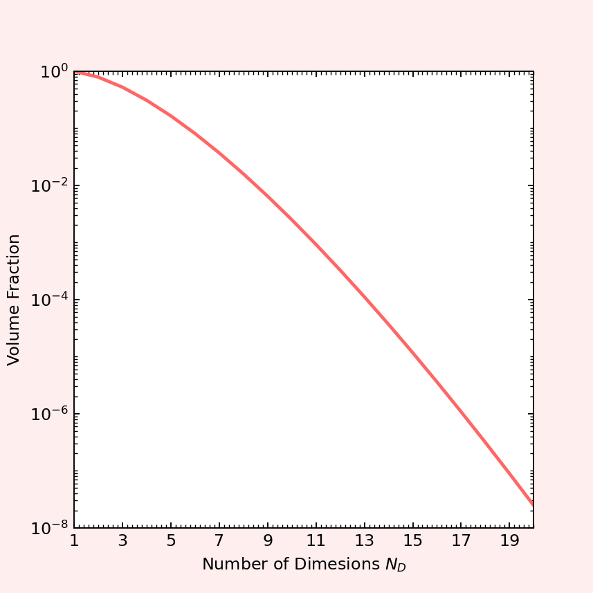
where $N_C$ is the normalization constant that is usually impossible to calculate analytically either because the functional form of $f(x)$ possess no analytic anti-derivative or the distribution is defined in high dimensions or both.

The MH algorithm pairs $p(x)$ with a known probability distribution $g(x)$ but in a way such that the algorithm ‘learns’ where to concentrate its effort by having $g(x)$ follow the current state around (in contrast to the accept-reject method where $g(x)$ is stationary).  At each step, the transition from the current state $a$ to the proposed or candidate next state $b$ happens according to the transition probability

\[ T(a \rightarrow b) = g(b|a) A(a \rightarrow b) \; , \]

where $g(b|a)$ is conditional draw from $g(x)$ centered on state $a$ (i.e., $g$ follows the current state around) and the transition probability $A(a \rightarrow b)$ is the MH decision step.  The right-hand-side of the transition probability directly maps $g(b|a)$ and $A(a \rightarrow b)$ to the first two and the last two sub-bullets of the execution step above, respectively. 

To derive the MH decision step correctly describes $A(a \rightarrow b)$, we impose detailed balance,

\[ p(a) T(a \rightarrow b) = p(b) T(b \rightarrow a) \; \]

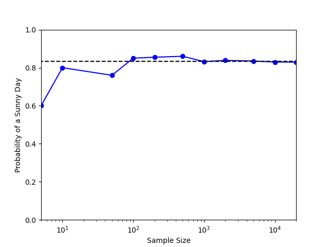
guaranteeing that the MCMC will eventually result in a stationary distribution.  That detailed balance give stationary distributions of the Markov chain is most easily seen by summing both sides over $a$ to arrive at a matrix analog of the stationary requirement ${\bar S}^* = M {\bar S}^*$ used in the Sunny Day Markov chain post.

The next step involve a straightforward plugging-in of earlier relations to yield

\[ \frac{f(a)}{N_C} g(b|a) A(a \rightarrow b) = \frac{f(b)}{N_C} g(a|b) A(b \rightarrow a) \; . \]

 Collecting all of the $A$’s over on one side gives

\[ \frac{A(a \rightarrow b)}{A(b \rightarrow a)} = \frac{f(b)}{f(a)} \frac{g(a|b)}{g(b|a)} \; . \]

Next define, for convenience, the two ratios

\[ R_f = \frac{f(b)}{f(a)} \; \]

and

\[ R_g = \frac{ g(a|b) }{ g(b|a) }  \; . \]

Note that $R_f$ is the ratio defined earlier and that $R_g$ is exactly 1 when the $g(x)$ is a symmetric distribution.

Now, we analyze two separate cases to make sure that the transitions $A(a \rightarrow b)$ and $A(b \rightarrow a)$ can actually satisfy detailed-balance. 

First, if $R_f R_g  < 1$ then detailed balance will hold if we assign $A(a \rightarrow b) = R_f R_g$ and $A(b \rightarrow a) = 1$.  These conditions mean that we can interpret $A(a \rightarrow b)$ as a probability for making the transition and we can then draw a number $q$ from a uniform distribution to see if we beat the odds $q \leq R_f R_g$, in which case we transition to the state $b$.

Second, if $R_f R_g \geq 1$ then detailed balance will hold is we assign $A(a \rightarrow b) = 1$ and $A(b \rightarrow a) = R_f R_g$.  These conditions mean that we can interpret $A(a \rightarrow b)$ is being a demand, with 100% certainty, that we should make the change.

These two cases, which comprise the MH decision rule, are often summarized as

\[ A(a \rightarrow b) = Min(1,R_f R_g) \; \]

or, in the case when $g(x)$ is symmetric

\[ A(a \rightarrow b) = Min\left(1,\frac{f(b)}{f(a)}\right) \; , \]

which is the form used in the algorithm listing above.

The last two columns explored the notion for transition probabilities, which are conditional probabilities that express the probability of a new state being realized some system given the current state that the system finds itself in.  The candidate case that was examined involved the transition probabilities of between weather conditions (sunny-to-rainy, sunny-to-sunny, etc.).  That problem yielded answers via two routes: 1) stationary analysis using matrix methods and 2) Markov Chain Monte Carlo (MCMC). 

The analysis of the weather problem left one large question looming.  Why anyone would ever use the MCMC algorithm when the matrix method was both computationally less burdensome and also gave exact results compared to the estimated values that naturally arise in an Monte Carlo method.

There are many applications but the most straightforward one is the Metropolis-Hasting algorithm for producing pseudorandom numbers from an arbitrary distribution.  In an earlier post, we presented an algorithm for producing pseudorandom numbers within a limited class of distributions using the Inverse Transform Method.  While extremely economical the Inverse Transform Method depends on the finding invertible relationship between a uniformly sampled pseudorandom number $y$ and the variable $x$ that we want distributed according to some desired distribution.

The textbook example of the Inverse Transform Method is the exponential distribution.  The set of pseudorandom numbers given by

\[  x = -\ln (1-y) \; , \]

where $y$ is uniformly distributed on the interval $[0,1]$, is guaranteed to be distributed exponentially. 

If no such relationship can be found, the Inverse Transform Method fails to be useful. 

The Metropolis-Hastings method is capable to overcoming this hurdle at the expense of being computationally much more expensive.  The algorithm works as follows:

• Setup
  • Select the distribution $f(x)$ from which a set random numbers are desired
  • Arbitrarily assign a value to a random realization $x_{start}$ of the desired distribution consistent with its range
  • Select a simple distribution $g(x|x_{cur})$, centered on the current value of the realization from which to draw candidate changes
• Execution
  • Draw a change from $g(x|x_{cur})$
  • Create a candidate new realization $x_{cand}$
  • Form the ratio $R = f(x_{cand})/f(x_{cur})$
  • Make a decision as the keeping or rejecting $x_{cand}$ as the new state to transition to according to the Metropolis-Hastings rule
    • If $R \geq 1$ then keep the change and let $x_{cur} = x_{cand}$
    • If $R < 1$ then draw a random number $q$ from the unit uniform distribution and make the transition if $q < R$

The bulk of this algorithm is very straightforward and simple.  The only confusing part is the Metropolis-Hastings decision rule in the last step and why it requires the various pieces above to work.  The next post will be dedicated to a detailed discussion of that rule.  For now, we’ll just show the algorithm in action with various forms of $f(x)$ which are otherwise intractable.

The python code for implementing this algorithm is relatively simple.  Below is a snippet from the implementation that produced the numerical results that follow.  The key points to note are:

• the numpy unit uniform distribution ($U(0,1)$) random was used for both $g(x|x_{cur})$ and the Metropolis-Hastings decision rule
• N_trials is the number of times the decision loop was executed but is not the number of resulting accepted or kept random numbers, which is necessarily a smaller number
• delta is the parameter that governs the size of the candidate change (i.e., $g(x|x_{cur}) = U(x_{cur}-\delta,x_{cur}+\delta)$
• n_burn is the number of initial accepted changes to ignore or throw away (more on this next post)
• x_0 is the arbitrarily assigned starting realization value
• prob is a pointer to the function $f(x)$

In addition to these input parameters, the value $f = N_{kept}/N_{trials}$ was reported.  The rule of thumb for Metropolis-Hastings is to have a value $0.25 \leq f \leq 0.33$.

x_lim    = 2.8
N_trials = 1_000_000
delta    = 7.0
Ds       = (2*random(N_trials) - 1.0)*delta
Rs       = random(N_trials)
n_accept = 0
n_burn   = 1_000
x_0      = -2.0
x_cur    = x_0
prob     = pos_tanh
p_cur    = prob(x_cur,-x_lim,x_lim)
 
x = np.arange(-3,3,0.01)
z = np.array([prob(xval,-x_lim,x_lim) for xval in x])
 
kept = []
for d,r in zip(Ds,Rs):
    x_trial = x_cur + d
    p_trial = prob(x_trial,-x_lim,x_lim)
    w       = p_trial/p_cur
    if w >= 1 or w > r:
        x_cur = x_trial
        n_accept += 1
        if n_accept > n_burn:
            kept.append(x_cur)

Two arbitrary and difficult functions were used for testing the algorithm:  $f_1(x) = |tanh(x)|/N_1$ and $f_2(x) = \cos^6 (x)/N_2$.  $N_1$ and $N_2$ are normalization constants obtained by numerically integrating over the range $[-2.8,2.8]$, which was chosen for strictly aesthetic reasons (i.e., the resulting plots looked nice).

The two parameters that had the most impact of the performance of the algorithm were the values of delta and x_0. The metric chosen for the ‘goodness’ of the algorithm is simply a visual inspection of how well the resulting distributions matched the normalized probability density functions $f_1(x)$ and $f_2(x)$.

Case 1 – $f_1(x) = |tanh(x)|/N_1$

This distribution was chosen since it has a sharp cusp in the center and two fairly flat and broad wings.  The best results came from a starting point $x_0 = -2.3$ over in the left wing (the right wing also worked equally well) and a fairly large value of $\delta=7.0$ was chosen such that $f \approx 1/3$.  The agreement is quite good.

A smaller value of $\delta$ lead to more samples being collected ($f=0.85$) but the realizations couldn’t ‘shake off the memory’ that they started over in the left wing and the results were not very good, although the two-wing structure can still be seen.

Starting off with $x_0 = 0$ resulted in a realization of random numbers that looks far more like the uniform distribution than the distribution we were hunting.

This result persists with smaller values of $\delta$.

Case 2 – $f_2(x) = \cos^6(x)/N_2$

In this case, the distribution has a large central hump or mode and two truncated wings.   The best results came from a starting value of $x_0$ at or near zero and a large value of $\delta$.

Lowering the value of $\delta$ leads to the algorithm being trapped in the central peak with no way to cross into the wings.

Finally, starting in the wings with a large value of $\delta$ leads to a realization that looks like it has the general idea as to the shape of the distribution but without the ability to capture the fine detail.

This behavior persists even when the number of trials is increased by a factor of 10 and no immediately satisfactory explanation exists.

In the last post, we demonstrated that not all conditional probabilities are conceptually equal even if they are linguistically equal.  The specific case discussed at the end – the sunny day case – doesn’t fit the usual mold.  To better understand why it doesn’t fit let’s looks back at the textbook case.

Ordinarily, we calculate a conditional probability by fixing one of the variables from a joint probability distribution and renormalizing so that ‘the probability of $B$ given $A$’, denoted by $P(B|A)$ obeys all the axioms of probability theory.  For simplicity, the joint probability distribution in the previous analysis was presented as a table (e.g. color and life of a bulb or snack preference based on sex) but any mathematically multi-variate function capable of being normalized serves.

But the sunny day case is different.  In that case, we define transition probabilities that express what the chance that the weather tomorrow will be like given the weather today, where there were only two possible outcomes: ‘Sunny’ (denoted as $S$) and ‘Rainy’ (denoted as $R$).  The conditional probabilities were:

\[ P(S|S) = 0.9 \; \]

and

\[ P(R|S) = 0.1 \; , \]

for the weather tomorrow based on today’s weather being sunny.  Likewise,

\[ P(S|R) = 0.5 = P(R|R) \; ,\]

 given that today is rainy.

It isn’t all clear how many actual variables we have in the joint probability distribution.  Is it 2, one for today and one for tomorrow?  Clearly that’s wrong since in any given span of days, say the month of September, taken in isolation, there are 28 days that serve as both a today and a tomorrow and 1 day each that is either a tomorrow or a today but not both.  As we’ll see below, in a real sense there are an infinite number of variables in the joint distribution since there are limitless todays and tomorrows (ignoring the obvious conflict with modern cosmology).

The question left hanging was just how could we determine the probability that, given an $N$-day long span of time, the weather on any given day was sunny.

This type of problem is called a Markov chain problem defined as the type of problem where the transition probabilities only depend on the current state and not something further back.  This type of system is said to have no memory.

There are two equally general methods for computing the long term probability of any given day being sunny or rainy but they differ in convenience and scope.  The first is the analytic method.

In the analytic method, we express the state of the system as a vector ${\bar S}$ with two components stating the probability of getting a sunny or rainy day.  The transition rules express themselves nicely in matrix form according to

\[ {\bar S}_{tomorrow} = M {\bar S}_{today} \; ,\]

which has the explicit form

\[ \left[ \begin{array}{c} S \\ R \end{array} \right]_{tomorrow} = \left[ \begin{array}{cc} 0.9 & 0.5 \\ 0.1 & 0.5 \end{array} \right] \left[ \begin{array}{c} S \\ R \end{array} \right]_{today} \; . \]

The explicit form of $M$ can be checked against an initial, known state of either ${\bar S}^{(0)} = [1,0]^{T}$ for sunny or ${\bar S}^{(0)} = [0,1]^{T}$ for rainy.

The matrix $M$ links the weather state today to that of tomorrow and we can think of it as an adjacency matrix for the following graph

with the interpretation that the edge weightings are the conditional transition probabilities.

Now lets place an index on any given day just to keep track.  The state of the n^th day is related to the initial state by

\[ {\bar S}^{(n)} = M {\bar S}^{(n-1)} = M^n {\bar S}^{0} \; .\]

Since we would like to know the probability of picking a sunny day from a collection of days, we are looking for a steady state solution, one which is immune to random fluctuations associated with a string of good or bad luck.  This special state ${\bar S}^{*}$ must correspond to $n \rightarrow \infty$ and so it must remain unchanged by successive applications of $M$ (otherwise it doesn’t represent a steady state).  Mathematically, this condition can be expressed as

\[ {\bar S}^{*} = M {\bar S}^{*}  \; , \]

or, in words, ${\bar S}^{*}$ is an eigenvector of $M$. Computing the eigenvectors of $M$ is easy with numpy and the results are

\[ {\bar S}^{*}_{\lambda_1} = [0.98058068, 0.19611614]^{T} \; \]

and

\[ {\bar S}^{*}_{\lambda_2} = [-0.70710678, 0.70710678]^{T} \; \]

for $\lambda_1 = 1$ and $\lambda_2 = 0.4$.  We reject the vector corresponding to $\lambda_2$ because it has negative entries which can’t be interpreted as probabilities.  All that is left is to scale ${\bar S}^{*}_{\lambda_1}$ so that the sum of the entries is 1.  Doing so gives,

\[ {\bar S}^{*} = [0.8333{\bar 3},0.16666{\bar 6}]^{T} \; ,\]

where the subscript has been dropped as it serves no purpose.

While mathematically correct, one might feel queasy about $\lim_{n\rightarrow \infty} M^n$ converging to something meaningful.   But a few numerical results will help support this argument. Consider the following 3 powers of $M$

\[ M^2 = \left[ \begin{array}{cc} 0.86 & 0.70 \\ 0.14 & 0.3 \end{array} \right] \; ,\]

\[ M^{10} = \left[ \begin{array}{cc} 0.83335081 & 0.83324595 \\ 0.16664919 & 0.16675405 \end{array} \right] \; ,\]

and

\[ M^{20} = \left[ \begin{array}{cc} 0.83333334 & 0.83333332 \\ 0.16666666 & 0.16666668 \end{array} \right] \; .\]

Clearly, repeated powers are causing the matrix to converge and the elements that obtain in the limit are the very probabilities calculated above and, by the time $n=20$ we have essentially reached steady state.

The second method is numerical simulation where we ‘propagate’ an initial state forward in time according to the following rules:

1. draw a uniform random number in the range $P \in [0,1]$ (standard range)
2. if the current state is $S$ then
   1. set the new state to $S$ if $P \leq 0.9$
   1. else set the new state to $R$
3. if the current state is $R$ then
   1. set the new state to $S$ is $P \leq 0.5$
   1. else set the new state to $R$
4. Record the new state and repeat

An alternative way of writing the same thing reads

1. draw a uniform random number in the range $P \in [0,1]$ (standard range)
2. if the current state is $S$ then
   1. set the new state to $R$ if $P \leq 0.1$
   1. else set the new state to $S$
3. if the current state is $R$ then
   1. set the new state to $R$ is $P \leq 0.5$
   1. else set the new state to $R$
4. Record the new state and repeat

Of course, hybridizations of these rule sets where block 2 in the first set if matched with block 3 in the second and vice versa also give the same results.  It is a matter of taste.

In any event, these rules are easy to implement in python and the following plot shows the fraction of $S$’s as a function of the number of times the rule has been implemented

The dotted line shows the value for the probability of a sunny day obtained from the first method and  clearly the simulations shows that it converges to that value.  This sunny/rainy day simulation is an example of Markov Chain Monte Carlo, which will be the subject of upcoming blogs.

It is an interesting aspect of human language that exactly the same wording can mean exactly different things, with each variation hiding subtle nuances of meaning and context.  This well-established principle makes human language expressive and evocative but also tends to obscure the channels of communication where precise communication is required.  Case in point, the use of conditional probability.

Consider the following two ‘cause-and-effect’ scenarios.  In the first, we survey two groups, each with 140 individuals, who are afflicted with similar diseases: a mild case of the flu and the common cold.  For our research purposes, we focus on only two of the set of symptoms common to both ailments and ask whether an individual complains more about having a sore throat or body aches.

Given the current statistics, medical community estimates that for a case of mild flu, patients rank the sore throat as more bothersome than body aches 57.14% of the time and body aches more bothersome 42.86% of the time.  The corresponding rankings for the common cold are 63.33% and 36.67% of the time for sore throat and body aches, respectively.

These rankings represent the conditional probabilities stating that if we know that an individual has a given disease then we should, within some statistical fluctuation, be able to say the probability that that individual will rank a sore throat ahead of body aches.  Alternatively, given a sample of patient, each known to have either a mild flu or the common cold, we should be able to say what proportion of them will rank which symptom as being worse.

To be concrete, consider that we have $N_f = 140$ people suffering with the flu and $N_c = 150$ with the common cold.  The proportions of these individuals that are predicted to rank the sore throat more would be given by the product of the conditional probability by the total size of the group.  Mathematically, the number of flu patients $N_{sf}$ ranking the sore throat as the primary problem is

\[ N_{sf} = P(s|f) N_f = 0.5714 \cdot N_f = 80 \; , \]

while the number of cold patients $N_{sc}$ agreeing that the sore throat is worse is

\[ N_{sc} = P(s|c) N_c = 0.4286 \cdot 140 = 60 \; . \]

In the same way, the number of flu and cold patients ranking body aches first can be obtained.  The results summarize nicely in the usual joint probability table we know from statistics

This is one way, and probably the most familiar way, of defining what is meant by conditional probability.  Other textbook examples involve surveying a population for attributes like the Christmas tree light example with the joint probability table

In order to follow what comes next, it is important to note that having the conditional probabilities is equivalent to having the table or vice versa.  Having the complete information represented in one form allows the unambiguous construction of the other.

Interestingly, there seems to be a case in which the term ‘conditional probability’ is used such that, as far as I can tell, the values can’t be meaningfully cast into table form like the above.  This case occurs when the use of the phrase ‘conditional probability’ is meant as a transition probability.  A textbook example of this is given in terms of the weather in the Wikipedia article on Examples of Markov Chains.

In this example, the conditional probabilities represent the chance that the weather tomorrow will be like the weather today.  For the sake of simplicity, the only two possible weather outcomes are ‘Sunny’ and ‘Rainy’.  The chance that it will be Sunny tomorrow given that it is Sunny today is 0.9.  Likewise, the chance that it will be Rainy tomorrow given that it is Sunny today is 0.1.  These facts are summarized in the conditional probabilities

\[ P(S|S) = 0.9 \; \]

and

\[ P(R|S) = 0.1 \; . \]

In a similar fashion, the conditional probabilities for a Sunny or Rainy tomorrow given that it is Rainy today are fifty-fifty

\[ P(S|R) = 0.5 = P(R|R) \; .\]

These conditional probabilities look, at first glance, to be on the same footing as the earlier ones.  The wording is the same; the notation is the same.  However, the interpretation is quite different.  The difference seems to lie in the fact that in the first case, the notion of having the flu or a cold and ranking which was worse, a sore throat or body aches, are underlying attributes of the sick individual.  In the second case, sunny or rainy weather is an attribute of the environment plain enough but the fact that there are an unlimited number of possibilities (e.g. SSRS for a four day sequence of weather with S = Sunny and R = Rainy) precludes making the usual table.

Mathematically, the heart of the difficult lies in the usual definition of a conditional probability in terms of sets.  For two possible outcomes $A$ and $B$ in a universe of possibilities the conditional probability that $B$ will occur given $A$ is

\[ P(B|A) = \frac{P\left( B \bigcap A \right)}{P(A)} \; , \]

where $P\left(B \bigcap A\right)$ is the probability of $A$ and $B$ occurring together (hence appearing in the joint probability distribution).  For example, in the Christmas tree light example above, the probability that a bulb chosen at random is both yellow and has a long life is

\[ P\left(long \bigcap yellow \right) = 0.0375 \; ,\]

while the probability of choosing a yellow bulb to begin with is

\[ P(yellow) = 0.15 \; . \]

The conditional probability given that the bulb is yellow that it also has a long life is

\[ P(long|yellow) = \frac{ P\left( long \bigcap yellow \right)}{P(yellow)} = \frac{0.0375}{0.15} =  0.25 \; . \]

So, we can move easily between conditional probabilities and joint probability distributions in this case.

In the case of the transition probabilities between weather, it isn’t clear how to encode the event $S$ as sunny today versus $S$ as sunny tomorrow.  The concepts of today and tomorrow are relative and constantly shifting during the passage of time.

One’s first reaction to that might be to not care.  But then how does one answer the simple question as to the proportion of days that are sunny?  This will be the topic of next month’s column.

This month we examine some of the specialized algorithms and packages that have been developed over several decades to perform importance sampling in a variety of scenarios.  Before digging to the specifics, it is worth setting the stage as to why importance sampling is such a key part of many problems.

A number of fields deal with high dimensional integrals.  Most likely, the original scenarios involving such integrals came about in connection to many-particle physics.  They arise in computing so-called loop corrections to quantum field theories which have the form

\[ I = \int d^3 k_1 d^3 k_2 \ldots d^3 k_n f({\vec k}_1, {\vec k}_2, \ldots ,{\vec k})_n \; , \]

where the ${\vec k}_i$ are the spatial momenta for the $i^{th}$ particle involved.  Likewise, the classical statistical description of the motion of group of $N$ particles involves computing the partition function given by

\[ Z = \int d^3 q_{(1)} d^3 p^{(1)} \ldots d^3 q_{(N)} d^3 p_{(N)} f(q^{i}_{(1)},p_{j}^{(1)},\ldots, q^{i}_{(N)},p_{j}^{(N)} ) \; , \]

where the $q^{i}_{(J)}$ and $p_{i}^{(J)}$ are the generalized coordinates and momenta for the $J^{th}$ particle and $f$ describes the interaction. 

In more recent years, high dimensional integrals have found a place in modeling images (ray tracing,  path tracing, and production rendering) and in mathematical finance, to name only a few.

Clearly, any system with sufficiently high number of continuous degrees of freedom is apt to birth an integral that has more dimensions than what can be efficiently dealt with using the more traditional structure quadrature methods – hence the need for Monte Carlo.  What is not so obvious is that, generically, the integrands are likely to be tightly peaked in only a small fraction of the total volume – hence requiring importance sampling.

This later point is typically easier to understand with a simple example in which we estimate the percentage of the volume of unit width consume by a sphere of unit diameter inscribed in the box.  In one dimension, the box extends over the range $[-0.5,0.5]$ and the sphere, defined as all the points within a distance of $0.5$ from the origin, are coincident.  The 1-sphere has two points where it touches the edge and there are no corners outside and thus it consumes 100% of the volume of the inscribing box.  In two dimensions, the box extends of the range $[-0.5,0.5]$ along two axes and the 2-sphere has volume $V = \pi (0.5)^2$.  There are four points where the 2-sphere touches the edge of the box and there are four corners that lie outside.  The 2-sphere only consumes 78.5% of the volume of the box.  In three dimensions, the volume of the 3-sphere is $V = 4\pi/3 (0.5)^2$ leaving 8 corners to lie outside and only 52.8% of the volume consumed.  A compact generalized formula for the volume of sphere in $N_D$-dimensions is given by

\[ V_{N_D} = \frac{\pi^{N_D/2}}{\Gamma \left(\frac{N_D}{2} + 1 \right)} \; .\]

The following plot shows just how quickly the volume fraction plummets to zero as the number of dimensions increases. 

At $N_D=20$ the 20-sphere touches all $2^20$ faces of the box but only at one point thus failing to include the $2^20$ corners containing points with distances greater than $0.5$ from the origin leading to an amazingly small percentage (0.0000025%) of the total volume occupied.  So, even in a scenario where the integrand seems ‘spread out’ the important region of the function is strongly peaked.

It is against this backdrop that we find several multi-purpose Monte Carlo importance sampling algorithms. 

Perhaps the oldest and most revered algorithm is VEGAS authored by G. Peter LePage in 1978.  VEGAS, which has its roots in particle physics, works by first ‘feeling out’ the integrand, looking for regions where the integrand is large in magnitude.  The algorithm grids the space coarsely to begin with and samples the function to make a histogram.  It then refines the sampling along each coordinate direction but avoids the combinatoric issues associated with structured quadrature by assuming that the integrand is separable in the sense that

\[ f(x_1, x_2, \ldots) = f_1(x_1) f_2(x_2) \ldots \; . \]

Having identified those regions with this adaptive gridding, VEGAS then concentrates the subsequent Monte Carlo trials using importance sampling to produce an estimate of the integral with an approximately minimized variance.

Roughly two decades after the release of VEGAS, Thorsten Ohl proposed an improvement to VEGAS in his paper entitled Vegas Revisited: Adaptive Monte Carlo Integration Beyond Factorization, in which he addresses the assumption that the integrand is separable.  Ohl found that his algorithm VAMP “show[ed] a significantly better performance for many ill-behaved integrals than Vegas.”  It isn’t clear how widely accepted VAMP has become but clearly some of the improvements that VAMP sought to add to VEGAS have been included in the new version of called VEGAS+.  Lepage’s article Adaptive Multidimensional Integration: VEGAS Enhanced describes the improvements in VEGAS+ over classic VEGAS, including a new adaptive stratified sampling algorithm.  Lepage provides both a free software python package on GitHub and comprehensive documentation.  Stratified sampling is a complementary method to importance sampling where the Monte Carlo samples are preferentially placed in regions where the integrand changes rapidly rather than strictly in regions where its magnitude is large.  The classic algorithm in stratified sampling is MISER but discussing it is out of scope in this analysis of importance sampling.  Suffice to say that both VEGAS and MISER are sufficiently important that they the only Monte Carlo algorithms packaged in the GNU scientific library.

In the last installment, we touched on the first rudiments of importance sampling as a way of improving the Monte Carlo estimation of integrals.  The key relationship is that a Monte Carlo estimate of an integral $I$ is given

\[ I = \int_a^b \, dx \, f(x) \approx \frac{1}{N} \sum_i \frac{f(x)}{p(x)} \pm \frac{\sigma}{\sqrt{N}} \; , \]

where $p(x)$ is a known probability distribution and $N$ are the number of Monte Carlo trials (i.e. random samples).

The error in the estimate depends on two terms: the number of Monte Carlo trials $N$ and the sample standard deviation $\sigma$ pulled at random from $p(x)$.  Although the error in the estimation can be made as small as possible by increasing the number of trials, the convergence is rather slow.  The importance sampling strategy is to make each Monte Carlo trial count as much as possible by adapting $p(x)$ to the form of $f(x)$ such that the ratio of the two terms is a close as possible to being a constant.

The examples of how to implement this strategy from the last post were highly contrived to illustrate the method but are not representative of what is actually encountered in practice since the majority of integrands are complicated and often no able to even be represented in closed form.

In this post, we are going to extend this method a bit by considering examples where the ratio of $f(x)/p(x)$ is not a constant.

Our first example will be to estimate the integral

\[ I = \int_{0}^{10} \, dx \, e^{-x^2} \; . \]

Up to an overall scaling this integral is proportional to the error function defined as

\[ erf(z) = \frac{2}{\sqrt{\pi}} \int_0^z \, dx e^{-x^2} \; . \]

While the error function is special function that can’t be expressed as a finite number of elementary terms, it has been studied and cataloged and, like the trigonometric functions, can be thought of as being a known function with optimized ways of getting a numerical approximation.  Our original integral is then

\[ I = \frac{\sqrt{\pi}}{2} erf(10) \approx 0.886226925452758 \; , \]

which we take as the exact, “truth” value.

To start we are going to estimate this integral using two different probability distributions: the uniform distribution, to provide the naïve Monte Carlo baseline for comparison, and the exponential distribution $p(x) \propto \exp(-x)$.  While the exponential distribution doesn’t exactly match the integrand (i.e. $exp(-x^2)/exp(-x) \neq \textrm{constant}$), it falls off similarly

and will provide a useful experiment to set expectations of what the performance will be when $p(x)$ only approximately conforms to $f(x)$.  Using the exponential distribution will also provide another change to use the variable substitution method for generating probability distributions. 

To generate an exponential distribution, we assume $y$ random variable related to the random variable $x$ through an integral where the exponential distribution is the integrand

\[ y = \int_{0}{x} \, dt e^{-t} \; .\]

Since $y$ is the cumulative distribution function it sits on the range $[0,1]$ and when it is uniformly distributed $x$ will be exponentially distributed.  The only remaining step is to express $x$ in terms of $y$.  For the exponential distribution, this is easily done as the integral is elementary.  Carrying out that integration gives

\[ y = \left. – e^{-t} \right|_{0}^{x} = 1 – e^{-x} \; .\]

Solving for $x$ yields

\[ x = -\ln (1-y) \; .\]

This relation is very simple to implement in python and a $N=10,000$ set of uniform random numbers for $y$ results the following histogram for the distribution for $x$,

which has a mean of $s_x = 1.00913$ and a $\sigma_x = 0.98770$ compared to the exact result for both being $1$.

Of course, most programming languages have optimized forms of many distributions and python is no different so we could have used the built-in method for the exponential distribution.  Nonetheless, following the above approach is important.  Understanding this class of method in detail reveals when it can and cannot work and illustrates some of the difficulties encountered in generating pseudorandom numbers from arbitrary distributions.  It helps to explain why some distributions are ‘built-in’ (e.g. the exponential distribution) when others, say a distribution proportion to a fifth-order or higher order polynomial over a finite range, are not.  It also provides a starting point for considering how to create distributions that are not analytically tractable.

With the exponentially-distributed pseudorandom numbers in hand, we can then estimate the integral with the importance sampling method and compare it to using naïve uniformly-distributed Monte Carlo.  The code I used to perform this comparison is:

Ns   = [i for i in range(10,2010,10)]
xmin = 0
xmax = 10
df   = pd.DataFrame()

#exact answeer for this integral in terms of the error function
exact = np.sqrt(np.pi)/2.0*special.erf(10) 

def f(x): return np.exp(-x*x)
def pu(span): return 1/(span[1]-span[0])
def pe(x): return np.exp(-x)
def xk(x): return -np.log(1-x)

for N in Ns:
    U = np.random.random((N,))
    FU = f(xmin + xmax*U)
    PU = pu((xmin,xmax))
    XK = xk(U)
    PE = pe(XK)
    FX = f(XK)

    mean_U = np.mean(FU/PU)
    sig_U  = np.std(FU/PU)/np.sqrt(N)
    err_U  = mean_U - exact
    mean_K = np.mean(FX/PE)
    sig_K  = np.std(FX/PE)/np.sqrt(N)
    err_K  = mean_K - exact

    row = {'N':N,\
           'I_U':mean_U,\
           'sig_I_U':sig_U,\
           'error_U':err_U,\
           'I_K':mean_K,\
           'sig_I_K':sig_K,\
           'error_K':err_K}
    df  = df.append(row,ignore_index=True)

Each record of the dataframe df contains the number of Monte Carlo trials $N$ as well as the estimated value of the integral, the uncertainty for both the uniform and importance-sampled estimators, and their corresponding actual error, respectively.  The following plot shows the error in the estimated value of the integral

clearly demonstrating the superior performance of the importance sampling with the exponential distribution, which converges rapidly for small $N$ and which exhibits less tendency to fluctuate as well.  The plot of standard deviation shows similar performance

with the standard deviation in the exponential sampling falling much faster as a function of $N$ and achieving a smaller and smoother overall value.  The standard deviation, which is the only measure one has when the exact value of the integral is unknown, is often called the formal error as it is taken as a proxy for the exact error.

Next month we’ll discuss some of use cases where the estimation of high-dimensional integrals necessitates importance sampling and the high-powered algorithms that can be plugged-in (sometimes with some effort).

The last post explored the error analysis for Monte Carlo integration in detail.  Numerical experiments indicated that the error in the algorithm goes as $1/\sqrt{N}$, where $N$ are the number of Monte Carlo trials used to make the estimate.  Further analysis of the sampling statistics led to a fundamental formula describing the estimated error of the estimated value $\langle I \rangle$ of the integral as

\[ \sigma_{\langle I \rangle } = \frac{\sigma}{\sqrt{N}} \; , \]

where $\sigma$ is the standard deviation of the random process used to evaluate the integral.  In other words, we could report the estimated value of some integral as

\[ I = \int_a^{b} \, dx f(x) \approx \frac{1}{N} \sum_{i} \frac{f_i(x)}{p_i(x)} \pm \frac{\sigma}{\sqrt{N}}  \; , \]

where $p(x)$ is some known probability distribution.  We report this estimate with the understanding that the last term is an estimated $1\sigma$ error of the sampling mean, which is expected to ‘look’ Gaussian as a consequence of the central limit theorem.

While it is attractive to think that an appropriate strategy to improve the estimate of $I$ is to crank up the number of Monte Carlo trials so that the error is as small as desired doing so completely ignores the other ‘knob’ that can be turned in the error equation, namely the value of $\sigma$.

At first, it isn’t obvious how to turn this knob and why we should even consider figuring out how.  Motivation comes when we reflect on the fact that in the most important and interesting cases the integrand $f(x)$ may be very or extremely computationally expensive to evaluate.  In those cases, we might look for a way to make every Monte Carlo trial count as maximally as it can.  Doing so may cut down on run times to get a desired accuracy from days to.

Given that motivation, the next question is how.  An illustrative example helps.  Consider the integral of a constant integrand, say $f(x)=2$ over the range $0$ to $1$ sampled with a uniform probability distribution.  The estimate of the integral becomes

\[ I = \int_0^{1} \, dx 2 \approx \frac{1}{N} \sum_{i} 2 = \frac{2N}{N} = 2 \; , \]

regardless of the number of trials.  In addition since each trial returns the same value, the sample standard deviation is $\sigma = 0$.  The estimate is exact and independent of the number of trials. 

Our strategy for the general $f(x)$ is quite clear; we want to pick the probability measure such that the ratio $f(x)/p(x) = \textrm{constant}$.  This strategy is termed importance sampling because the samples are preferentially placed in regions where $f(x)$ is bigger. This isn’t always possible but let’s examine another case where we can actually do this. 

Let’s estimate the integral

\[ I = \int_{0}^{1} \, dx \left(1 – \frac{x}{2} \right)  = \frac{3}{4} \; .\]

The integrand is linear across the range taking on the values of $1$ when $x=0$ and $1/2$ for $x=1$.  We want our probability distribution also be linear over this range but to be normalized.  A reasonable choice is to simply normalize the integrand directly, giving

\[ p(x) = \frac{4}{3}\left( 1 – \frac{x}{2} \right) \; .\]

The ratio $f(x)/p(x) = \frac{3}{4}$ and our expectation is that the Monte Carlo integration should give the exact result. 

The only detail missing is how to produce a set of numbers taken from that probability distribution.  To answer this question let’s follow the discussion in Chapter 8 of Koonin’s Computational Physics and rewrite the original integral in a suggestive way

\[ \int_0^{1} \, dx f(x) = \int_0^{1} \, dx \, p(x) \frac{f(x)}{p(x)} \; . \]

Now, define the cumulative distribution as

\[ y(x) = \int_0^x \, dx’ p(x’) \; \]

and make a change of variables from $x$ to $y$.  Using Leibniz’s rule,

\[ \frac{dy}{dx} = p(x) \; , \]

which gives $dx = dy/p(x)$.  Turning to the limits of the integral, we find $y(x=0) = 0$ and $y(x=1) = 1$ and the new form of the integral is

\[ \int_0^{1} \, dy \frac{f(y)}{p(y)} \; .\]

We can now tackle this integral by sampling $y$ uniformly over the interval $[0,1]$ as if the integral were originally written this way.   

Since $y$ is uniformly distributed, if an anti-derivative exist for $p(x)$ and we can invert the result to express $x=x(y)$ we will automatically get the desired distribution for random realizations of $p(x)$.  For the case at hand, $p(x) = \frac{4}{3}\left(1 – \frac{x}{2}\right)$.  The expression for $y$ is then

\[ y = \frac{4}{3} \left(x – \frac{x^2}{4} \right) \; .\]

This quadratic equation can be solved for $x$ to give

\[ x = 2- (4- 3y)^{1/2} \; .\]

The following figure shows the distribution of $x$ as a random variable given a 100,000 uniformly distributed random numbers representing $y$.

All of this machinery is easily implemented in python to provide a side-by-side comparison between directly sampling the original integral using both a uniform distribution and the importance sampling using the linear distribution.

import matplotlib as mpl
import numpy      as np
import pandas     as pd
import scipy      as sp
import matplotlib.pyplot as plt
Ns   = [10,20,50,100,200,500,1_000,2_000,5_000,10_000,100_000]
xmin = 0
xmax = 1
df   = pd.DataFrame()
def f(x): return (1.0 - x/2.0)
def w(x): return (4.0-2.0*x)/3.0
def x(x): return 2.0 - np.sqrt(4.0 - 3.0*x)
for N in Ns:
    y   = np.random.random((N,))
    Fu  = f(y)
    X   = x(y)
    Wx  = w(X)
    Fx  = f(X)
    row = {'N':N,'I_U':np.mean(Fu),'sig_I_U':np.std(Fu)/np.sqrt(N),\
          'I_K':np.mean(Fx/Wx),'sig_I_K':np.std(Fx/Wx)/np.sqrt(N)}
    df = df.append(row,ignore_index=True)
print(df)

The following table shows the results from this experiment (i.e. the contents of the pandas dataframe).

It is clear that the estimate of the integral $I_U$ slowly converges to the exact value of $3/4$ but that by matching the importance sampling weight $p(x)$ such that $f(x)/p(x)$ is a constant, we get an exact value $I_L$ of the integral with no uncertainty.

Of course, this illustrative example is not meant to be considered a triumph since we had to know the exact value integral to determine $p(x)$ in the first place.  But it does point to applications where we either don’t or can’t evaluate the integral. 

In the next post, we’ll explore some of these applications by looking at more complex integrals and discuss some of the specialized algorithms designed to exploit importance sampling.

The last post introduced the basic concept of Monte Carlo integration, which built on the idea of sampling the integrand in a structured (although random) way such that the average of the samples, appropriately weighted, estimates the value of a definite integral.  This method, while not as accurate for lower-dimensional integrals (for a given invested amount of computer time) as the traditional quadrature techniques (e.g., Simpson’s rule), really shines for problems in 4 or more dimensions.  (Note: The method also works well for multiple integrals in 2 and 3 dimensions when the boundary is particularly complex.)  This observation is based on the fact that the error in the Monte Carlo estimation goes as $1/\sqrt{N}$, $N$ being the number of samples, independent of the number of dimensions.

This post explores the error analysis of the Monte Carlo method and demonstrates the origin of the $1/\sqrt{N}$ dependence.

The first step is simply to look at how the error in the estimation of the integral varies as a function of the number of samples (hereafter called the number of Monte Carlo trials).  The example chosen is the polynomial

\[ f_p(x) = 3.4 x^3 -5.9 x^2 + 0.3 x -15.2 \; \]

used in the previous post.  The limits of integration are $x_{min} = -2$ and $x_{max} = 3.5$ and the exact value of this integral is $I_{p} = -68.46354166666669$.  The following table shows the error between the exact value and the value estimated using the Monte Carlo sampling method for the number of trials ranging from 100 to 100,000,000 trials.  All the data were obtained using a Jupyter notebook running python and the numpy/scipy ecosystem.

Even though the error generally trends downward as $N$ increases, there are fluctuations associated with the random nature of the sampling process.  The figure below shows a log-log scatter plot of these data along with a best fit line to the points.

The value of the slope returned by the linear regression was -0.529, very close to the expected value of $-1/2$; the $r^2$ value of the fit was 0.85 indicating that the linear fit very well explained the trend in the points, although it is important to realize that subsequent runs of this numerical experiment will produce different results.

While this result is compelling it lacks in two ways.  First, due to the random nature of the sampling, the trend will never be nailed down to be exactly an inverse square root.  Second, we had an exact value to compare to and so could quantitatively gauge the error.  In practice, we want to use the method to estimate integrals whose exact value is unknown and so we need an intrinsic way of estimating the error.

To address these concerns, we expand on the discussion in Chapter 10 of An Introduction to Computer Simulation Methods, Applications to Physical Systems, Part 2 by Gould and Tobochnik.  

In their discussion, the authors considered estimating

\[ I_{circ} = \int_0^1 dx \, 4 \sqrt{1-x^2}  = \pi \;  \]

multiple times using a fixed number of trials for each estimation.  Comparing the spread in the values of each estimation then gives a measure of the accuracy in the estimation.  To be concrete, consider the 10 estimations performed using 100,000 trials each.  The following table summarizes these cases with the first column being the average, the second the error against the exact value of $\pi$, (a situation, which, in general, we will not have).  The third channel is the standard deviation as measure of the spread of the sample used in the estimation.  We’ve introduced with hope of it filling the role of an intrinsic estimate of the error.

We can perform some statistical reduction of these data that will serve to direct us further.  First of all, the mean estimate (mean of the means) is $\langle I_{circ} \rangle = 3.1413985717765454$ with a standard deviation (sigma of the means) of $\sigma_{\langle I_{circ} \rangle} = 0.003304946237283195$.  The average of the standard deviation (mean of the sigmas) is $<\sigma>= 0.8930688485193065$.  Finally, the average error $<\epsilon> = 0.0027319130714524853$.  Clearly, $\sigma_{\langle I_{circ}\rangle} \approx <\epsilon>$ but both are two orders of magnitude smaller than $<\sigma>$.  A closer look reveals that the ratio $<\sigma>/\sigma_{\langle I_{circ}\rangle}$ is approximately $300 \approx 1/\sqrt{100,000}$.  This isn’t a coincidence.  Rather it reflects the central limit theorem.

The central limit theorem basically says that if we pull $K$ independent samples, each of size $N$, from an underlying population, then regardless of the structure of the population distribution (with some minor restrictions) the distribution of the $K$ averages computed will be Gaussian. 

This point is more easily understood with specific examples.  Below is a plot of the distribution of values of $4 \sqrt{1 -x^2}$ for a single Monte Carlo estimation with $N=100,000$ trials.  The histogram shows a distribution that strongly looks like an exponential distribution.

However, when this estimation is repeated so that $K=1,000$ and the distribution of those thousand means are presented in a histogram, the distribution looks strongly like a normal (aka, Gaussian) distribution.

The power behind this observation is that we can then estimate the error in original estimation in terms of the standard deviation of the sample itself.  In other words,

\[ \sigma_{\langle I_{circ} \rangle} =  \frac{<\sigma>}{\sqrt{N}} \; .\]

The proof of the generalize relation (Appendix 10B of Gould & Tobochnik) goes as follows.

Start with the $K$ independent samples each of size $N$ and form the $K$ independent means as

\[ M_k = \frac{1}{N} \sum_{n=1}^{N} x^{(k)}_n \; ,\]

where $x^{(k)}_n$ is the value of the $n^{th}$ trial of the $k^{th}$ sample.

The mean of the means (i.e. the mean over all $K \cdot N$ trials) is then given by

\[ {\bar M} = \frac{1}{K} \sum_{k=1}^{K} M_k = \frac{1}{K} \sum_{k=1}^{K} \frac{1}{N} \sum_{n=1}^{N} x^{(k)}_n \; .\]

Next define two measures of the difference between the individual measures and the mean of the means: 1) the $k^{th}$ residual, which measures the deviation of an $M_k$ from ${\bar M}$ and is given by

\[ e_k = M_k-{\bar M} \; \]

and 2) the deviation, which is the difference between a single trial and ${\bar M}$, is given by

\[  d_{k,n} = x^{(k)}_n – {\bar M} \; . \]

The residuals and deviations are related to each other as

\[ e_k = \frac{1}{N}\sum_{n=1}^{N} x^{(k)}_n – {\bar M} = \frac{1}{N} \sum_{n=1}^{N} \left( x^{(k)}_n – {\bar M} \right) =  \frac{1}{N} \sum_{n=1}^{N} d_{k,n} \; .\]

Averaging the squares of the residuals gives the standard deviation of the ensemble of means

\[ {\sigma_M}^2 = \frac{1}{K} \sum_{k=1}^{K} {e_k}^2 \;. \]

Substituting in the relation between the residuals and the deviations gives

\[ {\sigma_M}^2 = \frac{1}{K} \sum_{k=1}^{K} \left( \frac{1}{N} \sum_{n=1}^{N} d_{k,n} \right) ^2 \; .\]

Expanding the square (making sure to have independent dummy variables for each of the inner sums) yields

\[ {\sigma_M}^2 = \frac{1}{K} \sum_{k=1}^{K} \left( \frac{1}{N} \sum_{m=1}^{N} d_{k,m} \right) \left( \frac{1}{N} \sum_{n=1}^{N} d_{k,n} \right) \; .\]

Since the individual deviations are independent of each other, there should be as many positive as negative terms, and averaging over the terms where $m \neq n$ should result in zero.  The only surviving terms are when $m = n$ giving

\[ {\sigma_M}^2 = \frac{1}{K} \frac{1}{N^2} \sum_{k=1}^{K} \sum_{n=1}^{N} d_{k,n}^2 = \frac{1}{N} \left[ \frac{1}{KN} \sum_{k=1}^{K} \sum_{n=1}^N (x^{(k)}_n –{\bar M} )^2 \right] \; . \]

The quantity in the braces is just the standard deviation $\sigma^2$ of the individual trials (regardless to which sample they belong) and so we get the general result

\[ {\sigma_M} = \frac{\sigma}{\sqrt{N}} \; . \]

Next post will examine the implications of this result and will discuss importance sampling as a mechanism to drive the estimated error to a minimum.

It is a peculiar fact that randomness, when married with a set of deterministic rules, often leads to richness that is absent in a set of deterministic rules by themselves.  (Of course, there is no richness in randomness by itself – just noise).  An everyday example can be found in the richness of poker that exceeds the mechanistic (albeit complex) rules of chess.  This behavior carries over into the realm of numerical analysis where Monte Carlo integration presents a versatile method of computing the value of definite integrals.  Given the fact that most integrands don’t have an anti-derivative, this technique can be very powerful indeed.

To understand how it works, consider a function $g(x)$, which is required to be computable over the range $(a,b)$, but nothing else.  We will now decompose this function in a non-obvious way

\[ g(x) = \frac{f(x)}{p(x)} \; , \]

where $p(x)$ is a normalized function on the same interval

\[ \int_a^b dx p(x) = 1 \; . \]

If we draw $N$ realizations from $p(x)$

\[ x_1, x_2, \ldots, x_N \; \]

and we evaluate $g(x)$ at each value

\[ g_1, g_2, \ldots, g_N \; , \]

where $g_i \equiv g(x_i)$.

On one hand, the expected value is

\[ E[g(x)] = \frac{1}{N} \sum_i g_i \equiv {\bar g} .\]

This is the empirical value of the sampling of $g(x)$ according to $p(x)$. 

The theoretical value is

\[ E[g(x)] = \int_a^b dx p(x) g(x) = \int_a^b dx p(x) \frac{f(x)}{p(x)} = \int_a^b dx f(x) \; . \]

So, we can evaluate the integral

\[ I = \int_a^b dx f(x) \; \]

by sampling and averaging $g(x)$ with a sampling realization of $p(x)$.

The simplest probability distribution to consider is uniform on the range

\[ p(x) = \frac{1}{b -a} \; \]

and with $g(x) = (b-a) f(x)$ we can evaluate

\[ I = \int_a^b dx f(x) = \frac{1}{N} \sum_i g_i = \frac{b-a}{N} \sum_i f_i \; , \]

where $f_i \equiv f(x_i) $.

Before pressing on with the theory, let’s take a look at some specific examples.

For the first example, let’s look at the polynomial

\[ f_p(x) = 3.4 x^3 – 5.9 x^2 + 0.3 x – 15.2 \; \]

This function has the antiderivative

\[ F_p(x) = \frac{3.4}{4} x^4 – \frac{5.9}{3} x^3 + \frac{0.3}{2} x^2 – 15.2 x \; . \]

The integral of $f_p$ from $x_{min} = -2$ to $x_{max} = 3.5$ has the exact value

\[ \int_{x_{min}}^{x_{max}} dx f_p = F_p(x_{max}) – F_p(x_{min}) = -68.46354166666669 \; . \]

A simple script in python using numpy, scipy, and a Jupyter notebook was implemented to explore numerical techniques to perform the integral.  The scipy.integrate.quad function, which uses traditional quadrature based on the Fortran QUADPACK routines, returned the value of -68.46354166666667, which is exactly (to within machine precision) the analytic result.  The Monte Carlo integration, which is implemented with the following lines

N = 100_000
rand_x = x_min + (x_max - x_min)*np.random.random(size=N)
rand_y = f(rand_x)
I_poly_est  = (x_max - x_min)*np.average(rand_y)

returned a value of -68.57203483190794 using 100,000 samples (generally called a trial – a terminology that will be used hereafter) with a relative error of 0.00158.  This is not bad agreement but clearly orders of magnitude worse than the deterministic algorithm.  We’ll return to this point later.

One more example is worth discussing.  This time the function is a nasty, nested function given by

\[ f_n = 4 \sin \left( 2 \pi e^{\cos x^2} \right) \; , \]

which looks like

over the range $[-2,3.5]$.  Even though this function doesn’t have an anti-derivative, its integral clearly exists since the function is continuous with no divergences.  The deterministic algorithm found in scipy.integrate.quad generates the value of -2.824748541066965, which we will take as truth.  The same Monte Carlo scheme as above yields a value -2.8020549889975164 or relative error 0.008034.

So, we can see that the method is versatile and reasonably accurate.  However, there are two questions that one might immediately pose: 1) why use it if there are more accurate methods available and 2) can the estimates be made more accurate?  The remainder of this post will deal with answering question 1 while the subsequent post will answer the second question.

To answer question 1, we will cite, without proof, the answer to question 2 that states the error $\epsilon$ in the estimate of the integral goes to zero as the number of samples according to

\[ \epsilon \sim \frac{1}{\sqrt{N}} \; \]

independent of the number of dimensions. 

To determine the error for a conventional quadrature method (e.g. trapezoidal or Simpson’s), we follow the argument from Steve Koonin’s Computational Physics p 201.  Assume that we will evaluate the integrand $N$ times (corresponding to the $N$ times it will be evaluated with the Monte Carlo scheme).  The $d$-dimensional region over for the integral consists of a volume ${V} ~ {h}^d$.  Distributing the $N$ points over the volume means that the grid spacing $h ~ N^{-1/d}$. 

Koonin states that an analysis similar to those used for the usual one-dimensional formulae gives the error as going $O\left(h^{d+2}\right)$.  The total error of the quadrature thus goes as

\[ N O\left(h^{d+2}\right) = O\left(N^{-2/d}\right) \; .\]

When $d \geq 4$, the error in estimating the integral via Monte Carlo becomes smaller than that for standard quadrature techniques for a given computing time invested.  This reason alone justifies why the Monte Carlo technique is so highly favored.  In particular, Monte Carlo proves invaluable in propagating variations through dynamical systems whose dimensionality precludes using a gridded method like traditional quadrature.

The next post will derive why the Monte Carlo error goes as $1/\sqrt(N)$.

To start, this month’s column brings the experimental exploration of category theory from Lewvere’s and Schanuel’ book to an end.  Why?  Well, up to this point, the invested effort seems to be far larger than the gained benefit.  Category theory promises deep insight into more complex ideas – otherwise why would anyone study it – but the amount of effort required to get to that place in the text by Lewvere and Schanuel seems overwhelming.  There is no middle ground in their work.  Either it is painfully pedantic or deeply complex.

So, as a change of pace, this column will be returning to simpler, one-off topics.  For this month, I thought it would be interesting to share a thought about the overlap between philosophy and computer programming that came about from an interesting video.  In this video, Dave Farley of Constant Development discusses the history of computing paradigms with an eye towards the tribal standoffs between the object oriented crowd versus the functional programming adherents, with particular attention between the tribal standoffs between the two over which paradigm is best.

While it is both comforting and amusing is the Dave says that both positions are ‘rubbish’ (with a delightful accent no less).  I heartily agree with his basic point that one should pick the right paradigm for the right job.  Along those lines, the most insightful thing that he had to say is an observation he attributed to “Uncle” Bob Martin.  Martin, a computing pundit of some note, says the purpose of a programming paradigm to constrain us, to take away a degree of freedom that we had otherwise been allowed. 

After reflecting on this point on more than one occasion, I realized, even though Farley didn’t say this, that the idea of constraining the world as part of a paradigm is both an ontological and epistemological metaphysical process whose scope is far larger than just computer programming.  A paradigmatic way of thinking constrains the way we perceive reality by constraining how we divvy up the world around us into pieces we understand.

One of the earliest texts covering the idea of chopping up the world into useful chunks is found in the philosophical work of Aristotle entitled the Categories.  In this work, Aristotle lists 10 separate categories that that cover all the possible things that can be the subject of a proposition.  The work centers around language and how parts of speech reflect the ideas we hold and this ten-fold division was meant to encompass everything a person can think (or perhaps just talk) about.  While the work is useful, because it deals with common observations and mode of thought we all share, it is dense and sometimes difficult.  Mortimer Adler, in his book Aristotle for Everyone, calls it uncommon common sense.  Fortunately, the key point for this discussion is that Aristotle offers a paradigm (perhaps hard to grasp) that constrains how we think (or describe) the world.

A more prosaic example comes from our everyday experience of communicating with our fellow beings.  For example, many of us would consider the word ‘automobile’ to be straightforward to define and we expect that the dictionary entry would be non-controversial.  However, exactly how each of us thinks about ‘automobile’ depends on the paradigm being used. 

For a thermal engineer, whose livelihood centers on the study of work and heat, an automobile make conjure the concept of a gasoline or diesel engine, a drive chain and an exhaust.  He has constrained the world to one dealing with how energy is stored, how much of it can be stored in a given volume, and how it moves from place to place.  A systems engineer, whose livelihood derives from understanding the interplay of various technologies, would mostly see a car as a set of subsystems designed to interact appropriately.  Does the engine provide the necessary power to match the steering and suspension?  Does the fuel tank and milage match the intended purpose?  And so on.  Our systems engineer has constrained his view of the automobile in such a way ignores the details of thermodynamics and deals only with the abstract ways in which such subsystems interface with each other.  To an urban planner, the automobile represents an atomic entity whose characteristics and behaviors are constrained to be at the driving level.  Doing so, allows the urban planner to deal with matters of traffic congestion, proper placement of tolls, and the like without concerning himself with the way in which the automobile moves or how well it moves.

Now let’s returning to the question of computer programming paradigms.  Certainly, a programmer must know, when modeling an automobile, what level his solution must deal with.  Is he programming a finite-element thermal model, an abstract entity-relationship, or a stochastic Monte Carlo simulation to match the fictitious engineers of the previous discussion.  However, the interesting aspect of a seasoned programmer is that when thinking about programming paradigms in the abstract he is actually engaging in metaphysics.  He is not asking how to describe how a thing can be an automobile but how a thing can be.  The comparisons of various paradigms naturally leads to the study of being itself.  The computer programmer has to deal with not only the problem of deciding into what category the thing he is interested falls but also with the meta-problem of how to categorize the categorizations; how to pick between the various ways of abstracting and how to apply them to the ontology that is the world.

Farley raises another point that is worth pondering.  He believes that human beings are intrinsically classifying animals, even if he doesn’t phrase it quite that way.   For that reason, he believes that the object-oriented paradigm is more naturally matched to human thought.  However, his definition of object oriented programing as the marriage of data and behaviors with polymorphism as the constraint agent (each object owns its specific response to a common message like fall) does lead to some difficult ontological questions when modeling the physical world.  Does a rock know how to behave under the influence of gravity because it knows how to interpret the message sent from the Earth or does the Earth know how to make the rock fall because of a message that the rock sends, or is the message loop (i.e. the gravitational interaction) the key point?  Even though an exploration of this question is beyond the scope of this post the ability to pose this question shows the power of thinking about paradigms as constraints.

It is for this reason that I think programming will becoming increasingly more and more important component of our day-to-day lives; not just because of the practical applications involving our smartphones and tablets, our X-boxes and Play Stations, and our computers working to solve this problem or that, but because it will trigger in us a way to look at the world anew.   If only Aristotle could have lived to participate in these debates.