On the off chance that you, dear reader, are thinking that there is precious little overlap between the skeletons left over from dead fish and the high art of philosophy, let me set your mind at rest.  You are correct; there isn’t much.  Nonetheless, this installment isn’t a shortened quip-of-a-column designed to note this simple observation and then to make a quick, albeit graceful exit.  In point of fact, the fishbones that I am referring to have a great deal to do with philosophy, in general, and epistemology, specifically.

For those you aren’t aware, the fishbone or Ishikawa diagram (after Kaoru Ishikawa) is a way of cataloging the possible, specific causes of an observed event as a way of inferring which one is the most likely.  Its primary application is to those events where the effect is clearly and obviously identifiable but where the trigger of that event is unknown or, at least, unobservable.  One can usually find these diagrams applied in industrial or technological settings where a fault in a complex system rears its ugly head but the failure mode is totally or partially unknown.

Now it is one of those trendy nuggets of common knowledge that philosophy is one of those subjects designed for the technically-challenged to while away their time considering how many angels can dance on the head of a pin or whether to push the fat man onto the tracks in order to save the lives of the many passengers on the train.  No practical applications can be found in philosophy.  It has nothing important to offer workplaces where holes are drilled, sheet metal bent, circuits soldered, products built, and so on.

The fishbone diagram speaks otherwise – it deals with what is real and practical and with what we know and how we know it in a practical setting.  It marries concepts of ontology and, more importantly, epistemology with the seemingly humdrum worlds of quality assurance and manufacturing.

To appreciate exactly how this odd marriage is affected, let’s first start with a distinction that is made in fishbone analysis between the proximate cause and the root cause.  A practical example will serve much better here than any amount of abstract generalizations.

Suppose that as we are strolling through ancient Athens, we stumble upon a dead body.  We recognize that it is our sometime companion by the name of Socrates.  Having been fond of that abrasive gadfly and possessing a slice of curiosity consistent with being an ancient Greek, we start trying to determine just what killed Socrates.  One of us, who works in the new Athenian pottery plant where the emerging science of quality management is practiced, recommends making a fishbone diagram to help organize our investigation.

Inside the head of the fish we place the key observation that Socrates is dead.  Off the central spine, we string possible causes of death, grouped into categories that make sense to us.  After a lot of discussion, we agree these four:  Divine Intervention, Natural Causes, Accidental Death, and Foul Play.   Under each of these broad headings we add specific instances.  For example, some of us have heard rumors of the dead man’s impiety, so perhaps Zeus has struck him down with a thunderbolt.  Other suggest that being hit with a discus was the cause of death, just like what happened to uncle Telemachus at the last Olympic Games.  We continue on until we have our finished fishbone.

This version of the fishbone diagram aims at helping us determine the proximate cause.  We want to know what actually killed him without, at this stage, trying to figure out why (although the question of ‘why’ helped us in populating the list).

We then, in good logical fashion, start looking for observations that either strengthen or weaken each of the bones in our diagram.  We find no evidence of charring or submergence in water, so we argue that Divine Intervention is highly unlikely.  There is no blood or signs of blunt force trauma, so scratch all the possibilities under Accidental Death.  One of us notes that his belongings are all present and that his face is peaceful and his body shows no subtle signs of violence like what might be attributed to strangulation or smothering, so we think murder very unlikely.  Finally, one of us detects a faint whiff of a distinct odor and concludes that Socrates has died by drinking hemlock.

In fishbone analysis, hemlock poisoning is the proximate cause – the direct, previous link in the chain of causation that led to his death.  Note that we haven’t actually seen Socrates consume the lethal cocktail; we are simply inferring it based on the effect (he’s dead) and the smell (likeliest cause).  The next step is to determine the root cause – the reason or motivation for his consumption of the hemlock.

We find, after collecting a different type of observations, that he was executed by the Polis of Athens for impiety and for corrupting the morals of the youths of our city state.  We generally fill out this step by interviewing people and collecting human impressions rather than physical evidence.  A what point we decide that we’ve hit the root is up to us.  We can stop with the death sentence passed down by the Athenian court or we can look to the politics that led to that sentence.  We can stop with the politics or dig further into the social and demographic forces that led to Athenian democracy so disposed to dispatch the father of Western thought.  We can trace events back to Hippias the tyrant, or back to Homer, or wherever.

This sense of arbitrariness isn’t confined solely to where we cut off the determination of the root cause.  We also limited our universe of explanations in determining the proximate cause.  We can’t consider everything – how about dryads, sylphs, and satyrs?

In other words, all of us start our fishbone analysis with a Bayesian a priori expectation of likeliest causes and we apply, whether consciously or not, Occam’s razor to simplify.  Let’s reflect on this point a bit more.  Doing so brings into sharper focus the distinction between what we think we know, what we actually know, and what we don’t know; between the universe of knowable, unknown, and unknowable.  Ultimately, what we are dealing with is deep questions of epistemology masquerading as crime scene investigation.

The situation is even more interesting when one has an observable effect with no discernable cause.  Is the cause simply unknown or is it unknowable?  And how do we know in which category it goes without knowing it in the first place?

This epistemological division is even further muddied when we deal with indirect observations provide by tools (usually computers).  Consider the case where a remote machine (perhaps in orbit) communicates with another machine, which unpacks the electronic signals it receives.  If a problem is observed (a part is reported dead, for example), what does this actually mean?  Where does the fault lie?  Is it in the first machine or the second one?  Could the second one be spoofing by accident or malice (hacking) the fault on the first.  How does one know and where does one start?  And if one is willing to extend the concept of a second machine to include human beings and their senses then the line gets even more blurred between observer and observed.  Where does the fault lie, with our machines or with ourselves, and how does one know?

I will close on that note of uncertainty and confusion with an aporetic ending in honor of Socrates.  And all of it came from a little fishbone, whose most common practitioners would most likely tell you that they are not interested in anything so impractical as philosophy.

The concept of the Turing Test as the basic gate that an artificially intelligent system must pass to be judged sufficiently human-like is both pervasive and intriguing.   Dealt with widely in both serious academic circles and in fanciful science fiction avenues, the usual theme is one in which the AI must overcome a set of hurdles to pass the test.

Usually, these hurdles are viewed as a question of evolution – of smartening the AI so that it acts like a human being.  Topics along this line include enabling sophisticated algorithms that recognize levels of evocation; an essential property that allows for understanding humor, getting double entendres, recognizing sarcasm.  Poetry and evocative imagery is also a complication that has been explored off and on.

Far less frequently is the concept of devolution explored.  The idea here is to dumb down the AI so that it seems less like a computer and more like a human being.  It should know how to round numbers grossly, use vague characterizations, use contractions, cut verbal corners, and the like.  One should imagine Commander Data from Star Trek the Next Generation as the textbook example.

This post deals with an unillumined corner of this latter category.  Specifically, how to make sure an AI can mimic the intuition of a human being, warts and all.  What I am talking about is a designed AI with the same usual blind spots and foibles as the average human being. Nothing illustrates this so clearly as intuition-defying results that come from big numbers.

Humans are not usually good with numbers in general and are notoriously bad with big numbers.  This is such a prevalent problem that there is even a term to describe just how poor the average soul’s understanding of numbers and mathematics is – innumeracy.

Even for those practiced in the art, intuition can fail when big numbers come in the form of probability and statistics.  Two puzzles are famous for challenging the mortal mind:  The Birthday and the Monte Hall Puzzles.  Any AI that wants to blend in had better trip over these two problems with the rest of us or run the risk of being exposed as something other than human.

The Birthday Puzzle

Often called the Birthday Paradox, this puzzle is a significant challenge to the basic intuition that each of us has to the likelihood of coincidences.  As described, the Birthday Puzzle, goes something like this.  Suppose that there are $n$ persons in a room, say attending a party.  What is the probability that any two of them have the same birthday?  Stated slightly differently, how many people do you need in a room before the probability is 50% that any two of them share the same birthday.

To be concrete and to keep things as simple as possible, let’s agree to ignore leap days and the possibility of a birthday falling on February 29^th.  This step is not essential but it keeps the number of special cases to consider down to a minimum.

Ask the average person and they will tell you that you need about 182 people in the room to get a 50-50 shot (assuming that the average person can actually divide 365 in half and properly round).  Whether it is a result of nature or nurture, this ‘intuitive’ and ‘obvious’ answer is grossly wrong.

The easiest way to compute the probability is to compute the much easier probability that none of the $n$ persons have the same birthday and then to subtract this number from 1 to get the probability that at least one pair share a birthdate in common.

Suppose that there are 3 people in the room; then there are 365 days to assign person 1’s birthday, 364 days to assign to person 2’s birthday, and 363 days to assign to person 3’s birthday.  Each of these numbers is then divided by the total number of days to get the probability.  The value of this number is

\[ \tilde P = \frac{365}{365} \frac{364}{365} \frac{363}{365} \; . \]

The probability that in a group of 3 persons at least one birthday is held in common is

\[ P = 1 – \tilde P = 0.0082 \; .  \]

This approach, which doesn’t come naturally to most of us, is, at least comforting, in that common sense tells us that when there are 366 or more people in a room then at least one pair share a birthday.  The real assault on common sense begins when we generalize the analysis to an arbitrary number of people and graph the result.

The general formula is

\[ P_n = 1 – \frac{365}{365} \frac{364}{365} \cdots \frac{365-n+1}{365} \; .\]

When graphed the unexpected appears:  only 23 people are needed to get a probability just over 50%. 

By the time the number of people reaches about 60, the probability of a match is nearly 100%.  This result challenges our expectations and causes us genuine surprise.  How will an AI that passes the more conventional aspects of a Turing test react?

The Monte Hall Puzzle

Even more interesting and non-intuitive is the Monte Hall or Let’s Make a Deal Puzzle.  Based on the final segment of the game show Let’s Make a Deal, contestants are offered a choice between three doors.  Behind two of them are so-called booby prizes, usually a farm animal or some other unwanted thing.  Behind one of the doors is usually a car.  Monte Hall, the host of the show, asks the contestant to pick one door.  Next, he opens one of the other two doors and reveals one of the booby prizes (e.g. the goat).

Monte’s final step is to offer the one unopened door in trade to the contestant.  The question then is should the contestant accept the offer and switch doors or should he stay with his original pick?  Of course, there is no way to guarantee the correct choice, but the contestant has a definite statistical advantage if he switches.  The probability that the car is behind the door he chose is 1/3 while the probability it is behind the other door is 2/3.  Most people see two doors and assume that the odds are 50-50.  That’s human intuition – even though it is wrong.  And Monte Hall, who I believe must have been a confidence man before going legit, played on the contestant’s greed and excitement, by offering cash if they stay with their first choice.  Usually, he kept them from getting the car, which I suppose was his aim.

Now imagine what would happen when an AI went onto Let’s Make a Deal.  Certainly, the AI should be able to understand natural language.  But how should it react to the door choices, to Monte Hall’s con-man techniques.  If the AI is going to fool the humans around it, it’d better be conned alongside the rest of us.

Imagine that it’s Christmas Eve and, due to some poor planning on your part, you find yourself short of a few gifts – gifts for key people in your life.  You reckon that you have no choice but to go out to the mall and fight all the other last minute shoppers to find those special trinkets that will bring smiles to all those faces you would rather not look at when they are frowning.  You know parking will be a delicate issue with few choices available at any given time and, as you enter the lot, you happen to see a space about one foot shy of a football-field’s distance to the mall entrance.  Should you take it or is there a better one closer?

If you take the space, you are in for a long walk to and fro as well as a waste of your time – and maybe, just maybe, the gifts will be gone by the time you get there.  If you pass by the space you run the risk of not finding a closer space and, most likely, this space will not be there when you circle back.

In a nutshell, this type of problem is best described under the heading ‘knowing when it is time to settle’.  It has broad applications in wide ranging fields; any discipline where decision making is done within the context of uncertainty mixed with a now-or-never flavor falls under this heading.

Within the computing and mathematical communities, this scenario is dubbed The Secretary Problem and has been widely studied.  The article Knowing When to Stop by Theodore Hill, published by The American Scientist, presents a nice introduction and discussion of the problem within many of the real world applications.  The aim of this month’s column is to look at some realizations of the problem within a computing context, and to look at some variations that lead to some interesting deviations from the common wisdom.  The code and approach presented here are strongly influenced by the article The Secretary Problem by James McCaffrey in the Test Run column of MSDN Magazine.  All of the code presented and all of the results were produced in a Jupyter notebook using Python 2.7 and the standard suite of numpy and matplotlib.

The basic notion of the Secretary Problem is that a company is hiring for the position of secretary and they have received a pool of applicants.  Since it is expensive to interview and vet applicants and there is a lost opportunity cost for each day the position goes unfilled, the company would like to fill the position as soon as possible.  On the other hand, the company doesn’t want to settle for a poor candidate if a more suitable one would be found with a bit more searching.  And, overall, what expectations should the company have for the qualifications of the secretary; perhaps the market is bad all over.

Within a fairly stringent set of assumptions, there is a way to maximize the probability of selecting the best choice by using the 1/e stopping rule.  To illustrate the method, imagine that 10 applicants seek the position.  Divide the applicant pool up into a testing pool and a selection pool, where the size of the testing pool is determined (to within some rounding or truncation scheme) by dividing the total number of applicants by e, the base of the natural logarithms. Using truncation, the testing pool has 3 members and the selection pool has 7.

The testing pool is interviewed and the applicants assessed and scored.  This sampling of the applicant pool serves to survey the entire pool.  The highest score from the testing pool sets a threshold that must be met or exceeded (hopefully) by an applicant within the additional population found in the selection pool.  The first applicant from the selection pool to meet or exceed the threshold is selected; this may or may not be the best overall candidate. Following this approach, and using the additional assumption that each applicant is scored uniquely, the probability is 36.8% chance of getting the best applicant (interestingly, this percentage is also 1/e).

This decision-making framework has three possible responses:  it can find the best applicant, it can settle on a sub-optimal applicant, or it can fail to find any applicant that fits the bill.  This later case occurs when all the best applicants are in the Testing Pool and no applicants in the Selection Pool can match or exceed the threshold.

To test the 1/e rule, I developed code in Python within the Jupyter notebook framework.  The key function is the one that sets up the initial applicant pool.  This function

def generate_applicants(N,flag='uniform'):
    if flag == 'integer':
        pool = []
        for i in range(0,N):
            pool.append(np.random.randint(10*N))
        return np.array(pool)
    if flag == 'normal':
        temp          = np.abs(np.random.randn(N))
        return np.floor(temp/np.max(temp)*100.0)/10.0
    if flag == 'uniform':
        return np.floor(np.random.rand(N)*100.0)/10.0
    else:
        print "Didn't understand your specification - using uniform distribution"
        return np.floor(np.random.rand(N)*100.0)/10.0

sets the scores of the applicants in one of three ways.  The first method, called ‘integer’, assigns an integer to each applicant based on a uniform probability distribution.  The selected range is chosen to be 10 times larger than the number of applicants, effectively guaranteeing that no two applicants have the same score.  The second, called ‘normal’, assigns a score from the normal distribution.  This approach also effectively guarantees that no two applicants have the same score.  The occasions where both methods violate the assumption of uniqueness form a very small subset of the whole.  The third method, called ‘uniform’, distributes scores uniformly but ‘quantizes’ the score to a discrete set.  This last method is used to test the importance of the assumption of a unique score for each applicant.

A specific applicant pool and the application of the 1/e rule can be regarded as an individual Monte Carlo trial.  Each trial is repeated a large number of times to assemble the statistics for analysis.  The statistics comprise the number of times the best applicant is found, the number of times no suitable applicant is found, and the number of times a sub-optimal applicant is found and how far from the optimum said applicant is.  This last statistic is called the settle value, since this is what the company has had to settle for.

The following figure shows the percentage of times that each method finds an optimal candidate from the selection pool by using the 1/e stopping rule.

Note that for the two methods where duplication is nearly impossible (integer and normal), the percent of total success remains, to within Monte Carlo error, at the theoretically derived value of about 36.8 %.  In contrast, the uniform method, which enjoys a quantized scoring system, shoots upwards to a total success rate of 100%.  The reason that explains this behavior is that with a quantized scoring system there is only a discrete set of values any applicant can achieve.  Once the number of applicants gets great enough, the testing pool perfectly characterizes the whole.   And while the number of applicants needed to achieve this higher percentage is impractical for finding a secretary (who really wants 640 applicants interviewing for the position) the application to other problems is obvious.  There is really no reason that a decision process should always hinge on the difference between two choices of less than a fraction of the overall score.  This fact also explains why businesses typically ‘look’ at the market and pay careful attention to who is hiring whom.

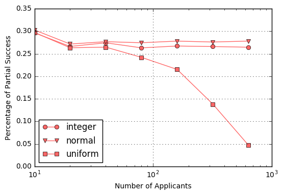
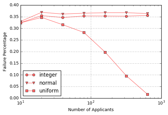
For completeness, the following figures show the analogous behavior for the partial success percentage

and the total failure scenarios

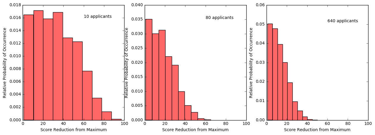
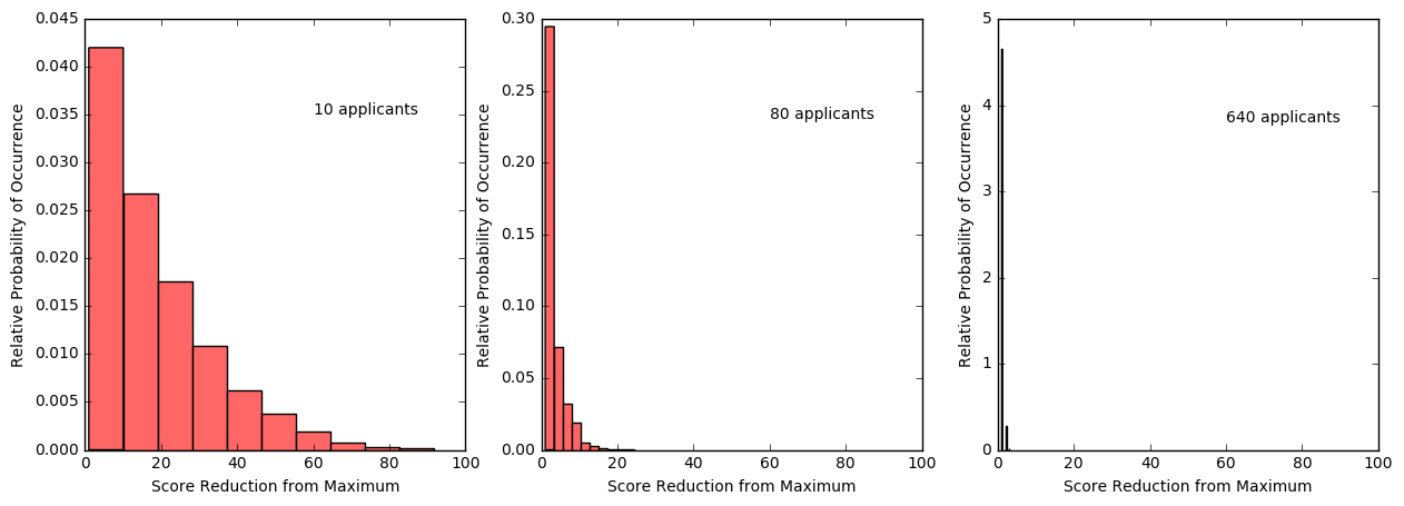
An interesting corollary is to ask, in the case of partial success, how much short of optimal did the decision process fall in the process of settling on a sub-optimal selection.  The following figures shows histograms for 10, 80, and 640 applicants in the applicant pool for those cases where the decision process had to settle for a sub-optimal choice, for the normal and uniform cases, respectively.  As expected, there is an improvement in how far from the maximum the decision falls as the testing pool size increases but, even with 640 applicants, the normal process has a significant probability of falling short by 20% or more.

In contrast, the distribution for the uniform scoring quickly collapses, so that the amount that the settled-upon candidate falls from the optimum is essentially within 5% even with a moderately sized applicant pool.  Again, this behavior is due to the quantized scoring, which more accurately reflects real world scenarios.

At this point, there are two observations worth making in brief.  First, the core assumption of the original problem, that all applicants can be assigned a unique score, is worth throwing away.  Even if its adoption was crucial in deriving the 1/e stopping rule, real world applications simply do not admit a clear, unambiguous way to assign unique scores.  Second, it is, perhaps, astonishing how much richness is hidden in something so mundane as hiring a qualified candidate. Of course, this is to be expected, since good help is hard to find.

It has been some time since this column explicitly examined the great Philosopher or explicitly cited his philosophy.  And while his approach to thinking and reflecting on various problems has never been far from the matters usually discussed here, I’ve not actually invoked his name for many columns.  So, it may seem to be a bit of a surprise to start the new year by mentioning Aristotle and whiskey together in this month’s title.  To some it may even be viewed as an unforgivable irreverence to one of the world’s greatest thinkers.  But, as I hope to show, there is nothing irreverent or surprising in linking Aristotle to alcoholic spirits, beyond the usual association that many have about the ancient Greeks – an expectation, no doubt, largely set by Plato’s Symposium.  At issue is the Aristotelian concept of virtue, the sloppy practice of equivocation (double-speak) in logical arguments, and a somewhat famous speech about whiskey made by Noah ‘Soggy’ Sweat Jr.

In 1952, a Mississippi’s law-maker by the name of Noah ‘Soggy’ Sweat Jr., was asked about his position regarding the state’s continued prohibition on selling alcoholic beverages to its citizens.  Soggy’s speech, which has since become immortalized due to its colorful language and its terseness, reads as

The standard analysis found at Wikipedia or at Bo Bennett’s Logically Fallacious website is that Soggy’s rhetoric is an amusing example of double-speak.  Bennett has the following to say about this speech:

On the surface, Bennett’s analysis seems to be spot on; Soggy’s speech suggests double-talk of the highest order uttered, most likely, with that old, rolling, Southern voice best exemplified by Foghorn Leghorn.  But there is another interpretation that is equally valid and should be explored, in the spirit of fairness.

To understand this more charitable interpretation, we need to step back and understand the Aristotelian concept of virtue; a concept discussed by Aristotle in many places, most notably in Book II of the Nicomachean Ethics.

The concept of virtue coincides with the proper balance between an excess or a deficiency of trait.  In the case of courage or bravery, Aristotle would say that the virtue of courage is having the proper mix between the two extremes of courage.  On one side, the soldier who possesses too little courage is timid and is incapable of performing his function in battle or even, most probably, even incapable of saving his own life.  On the other, the soldier who jumps into danger with no thought whatsoever for his safety or those of his compatriots serves no useful purpose due to his rashness and foolhardiness.

The Aristotelian notion of virtue as the balance between two extremes can be applied to Soggy’s speech as well.  At one extreme, is his first meaning of ‘by whiskey’: the overindulgence in alcohol that weakens character, causes lapses in judgement, and dissipates wealth, prosperity, and family cohesion.  This extreme is drunkenness indulged in by the alcoholic and should be avoided.

The other extreme is a bit more difficult to identify precisely because Soggy refers to it obliquely by noting all the advantages that result from its avoidance rather than discussing all the ills that follow by its pursuit.  This extreme, which may be called prudishness or uptightness, is often the province of the teetotaler, who deprives himself of the benefits that follow from the proper use of wine and spirits.  History shows that almost all cultures reserve an honored spot for ‘adult beverages’ because of the good effects they bring to both the body and the soul of its citizens.  In addition, Soggy points out that their production forms a significant sector of the modern economy, resulting in gainful employment and ample tax revenues that are also beneficial to society.

So there are at least two readings of Soggy’s speech: the first looks at it as a crass example of political jibber-jabber, the second credits it as a colorful explanation, in layman terms, of the virtue of alcohol.  Personally, I prefer the latter interpretation as it brings the great philosophical thought of ancient Greece to the everyday political doings of the modern world.

The scope of human knowledge has certainly changed over the last 3000 years.  Daily, we manipulate electrons and beam electromagnetic signals to and fro.  Large scale distribution networks move goods between highly specialized production centers.  Information flows from one corner of the globe to another in a matter of seconds.  Clearly, we live in an age of wonder.  But interestingly, while what we have learned has increased over the centuries, the methods of inquiry into obtaining new knowledge really haven’t changed all that much; certainly what we know has changed greatly but not how we learn it.

Case in point, it the use of regression or recursion as a tool for understanding the world in a philosophical way.  The applications of this approach are numerous due to the wide utility and the fruitful applications of it.

For example, Aristotle argued for that Man must have a purpose by using a type of regression argument whose spirit, although not its explicit nature, goes something like this.  Consider the bones of the hand; their function is to provide stiffness.  Likewise, the ligaments, tendons, and muscles provide the articulation.  The nerves provide the sense of touch and the flesh provides a means of touching, gripping, and holding as well as a unity and an encapsulation for the other parts.  All of these pieces have a function to perform in the greater existence that is the hand.  Likewise, one can find smaller parts serving limited roles within limbs, organs, and systems within the human body:  the eye serves to see; the nose to smell and breath; the mouth to chew, taste, drink, eat, breathe, and talk; and so on.  Since each piece contributes, through its function, to the greater function of the thing to which it is a part, isn’t reasonable to assume that the completed whole, the sum of all these individual parts within parts, also has a function or purpose?  This argument, put forward approximately 2500 years ago, is still compelling and persuasive.

Saint Thomas Aquinas, one the great philosophers of the medieval world, put forward arguments greatly influenced and cast in the form of Aristotle’s arguments.  In his Cosmos section of the Summa Theologica, Aquinas offers five proofs for the existence of God based on the concept of regression.  In outline form they are:

In all of these arguments, Aquinas identifies the thing that prevents an infinite regress, that stops the chain of thinking at a well-defined point, as God.

These kinds of logical arguments are not limited to the purely metaphysical realm.  One of the crowning achievements of mathematics is the development of set theory, which depends heavily on the type of arguments put forward above.  The presence of a run-away regress, one that never stops, is a sign of issues within set theory.  This typically, although not exclusively, happens when dealing with infinite collections or sets of things and leads to many paradoxes that must be resolved in order for mathematics to be put on a firm foundation.

Perhaps the most famous example is Russell’s paradox.  The paradox is based on defining two types of sets:

It isn’t at all clear that extraordinary sets exist.  If they do, they can’t be constructed using finite sets or the more familiar infinite sets like the integers or reals.  But assuming that they do exist, one can ask the following question:

To see that this leads to a paradox, first suppose that this set, call it Q, doesn’t contain itself.  It is then an ordinary set by definition.  Since it is ordinary, it should go in a listing of all ordinary sets – that is, it should contain itself.  Thus, we conclude that Q is extraordinary (hence the need to define the term in the first place).

So far so good!

But the fly in the ointment comes when we look carefully at Q being extraordinary.  The membership requirement to be in Q is that the element must be ordinary.  But if Q is contained within Q, it must be ordinary.  And so, we arrive at an infinite loop where one condition implies the other and vice versa.

Oddly enough, even though the trappings are associated with present-day set theory, replete with fancy modern symbols, the structure is almost the same as the ancient liars paradox.  The main ingredients are self-reference and a requirement to end an infinite regression.

The solution of these paradox is a story for another post.  The point here is that while the physical tools we use to manipulate the world have evolved dramatically over the centuries, the mental tools we use to grapple with logic remain largely unchanged.

Last month’s column explored the surprising complexity that results from the repeated application of the simple set of rules called the Half or Triple-Plus-One (HTPO).  Despite the fact that the rules are easy to understand and apply, composing their application iteratively led to rich patterns that defy the ability of the current state of mathematical logic to fully predict or prove.  So it should come as no surprise that there similar systems exhibit ‘big things in small packages’ behavior.

One class of systems where the application of simple local rules leads to complex global behavior is known as cellular automata.  These systems are usually modeled as living on a grid or lattice usually with a rectangular topology, although other connection schemes exist.

The state of the system is specified by a discrete state variable living at the grid point, with the most common state being specified by the integers 0 or 1, corresponding to ‘on’ or ‘off’.  The transition rules for deciding whether a grid point turns from on to off or vice versa are usually based on the local neighborhood of the grid point and are usually specified by relatively simple rules.

As in the HTPO case, the fun begins when the entire system dynamics for extended systems are taken into account.  Even though a specific grid point only interacts directly with its neighbors (the precise definition of what these are differ from system to system) its future evolution is determined by its neighbor’s interactions with their neighbors and so on.  In a real sense, local rules propagate out globally, and this is how the complexity results.

Perhaps the best known and popular cellular automaton system is Conway’s Game of Life.  This system takes place on a rectangular grid with the state of the system specified by 0 for off (‘dead’) and 1 for on (‘alive’).  Each cell has 8 neighbors, the closest cells to the north, north-east, east, south-east, south, south-west, west, and north-west.  The rules for how a particular grid cell evolves in time are:

• If a cell is alive and has less than 2 neighbors, it dies from heart-crushing loneliness and a failure by society-at-large to meet its needs,
• if a cell is alive and has 2 or 3 neighbors, it flourishes due to a balanced social life where it is integrated properly into society,
• if a cell is alive and has 4 or more neighbors, it dies from overcrowding, squalor, and disease,
• and if a cell is dead but there are exactly 3 neighbors, a new baby is born to settle into the empty spot.

Of course, none of the colorful language used above is canonical.  John Horton Conway picked the rules to try to balance the birth and death rates such that there would be no explosive growth and that the outcomes were not trivially predictable from the inputs.  According to the Wikipedia article linked above, Conway’s work was motivated by the desire to simplify von Neumann’s invention of a computational ‘machine’ that could build copies of itself.

The introduction of the Game of Life in 1970 sparked an entire industry due to the rich, emergent patterns that result.  To give a taste of the possibilities consider some simple configurations on a 6×6 grid.  Perhaps the simplest, non-trivial configuration is the block, which consists of 4 cells clustered together.

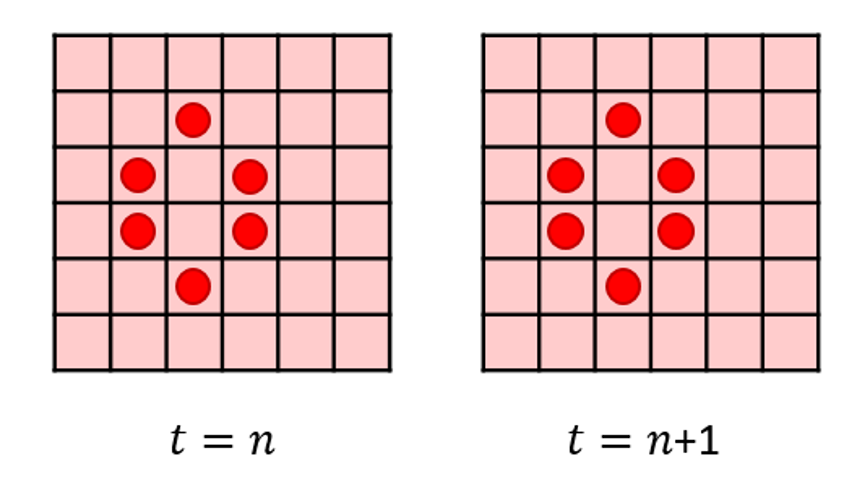
Since each cell has 3 neighbors, the pattern, once established, persists into eternity and the four cells live forever together in a stable colony.   Interestingly, this future-time stability does not imply past-time stability as this configuration can be reached by a variety of enormously dynamic and turbulent pasts as long as the penultimate step is a 3-cell ‘L’ configuration.

There are many stable configurations like the block.  Another one that tends to appear in simulations is the beehive, which also lasts from one time to another time unless disturbed.

It is interesting to note that the addition of one extra cell anywhere where it may be counted as a neighbor to the beehive ruins the stability completely.

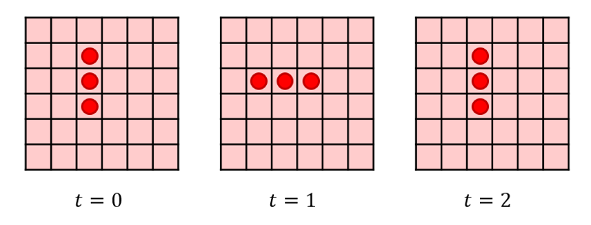
Dynamic patterns that have a stable form (really stationary) are also present, some of which are periodic and others which exhibit non-periodic, complex motions.  The simplest examples of periodic behaviors are those structures that seem to spin or rotate thus seeming to retain their shape.  The textbook example of this is the blinker that appears to rotate.

A more careful analysis shows that only the central cell persists while the exterior ones die and resurrect every second time step.  The Wikipedia article shows other periodic structures, including the very beautiful pulsar, that exhibit much more complex periodicities.

In the class of non-periodic stationary structures comes the glider, which is a 5-cell structure that sort-of shuffles its way across the board so that it walks through 4 distinct shapes such that its center moves one cell diagonally every 4 steps.

Obviously, a huge amount of complexity results from these simple rules.  But the Game of Life has more structure than the emergence of a bewildering array of patterns.  It turns out all logic gates needed in computing can be constructed using gliders, as seen in this video by Alex Bellos

The key structure for producing the gliders is known as Gospar’s Glider Gun, which pumps out a signal (a glider) that can be interrupted by other gliders from other guns.  The fact that all possible logic gates can be constructed in the Game of Life means that it is Turing-Complete.  Thus you can program any algorithm in Game of Life, including the Game of Life

Amazing what a few simple rules can do!

Big things come in small packages.  From tiny acorns grow mighty oaks.  Never judge a book by its cover.  These familiar euphemisms try to capture, in a pithy way, the basic idea that simple looking systems can often hide a surprising amount of complexity.   This basic observations couldn’t more true than in the case of the Collatz Conjecture.

The Collatz Conjecture is so simple that, on the face of it, it must be easy to prove.  But like other easily stated suppositions in mathematics, the proof, if one exists, must be particularly difficult to construct, since it has eluded mathematicians for nearly 100 years.

In a nutshell, the Collatz Conjecture says that a particular process, described just below, when repeatedly applied to any integer always ends up the same way, regardless of the starting value of the integer.  The process, referred to as the Half or Triple-Plus-One (HTPO) process, is as follows:

There it is.  It is so simple that it can be implemented in a few lines in just about any language; probably even in COBOL.  And yet, proving that this conjecture is actually so hard that the famous mathematician Paul Erdös is credited with saying

Obviously this column is not going to present a proof but it is going to explore some of the properties of the conjecture – including a few that may not have been seen in the literature.  There are two reasons for doing so.

The first reason is the sheer joy and delight that arises from seeing inexplicable complexity arise out of such simple rules.  Amazingly rich plots results simply by looking at the data from numerical experiments in a variety of different ways.  What, at first, may look like randomness resolves itself in patterns later on as the number of integers examined is increased.

The second reason is less about mathematics and far more about human reason.  Why a proof is hard to find is a topic in epistemology worth exploring all on its own.  Consider that the Collatz conjecture is a system that is far easier to encode in a computer than say the solution to an orbital mechanics problem or the motion of a fluid over a fixed object like an airplane wing.  No calculus or linear algebra is required.  Nowhere does one need real or complex numbers.  All the machinery that is needed is learned in elementary school and yet the proof is much harder than those associated with the ‘more advanced’ topics.  Surely there is a Socratic lesson buried in all of this. But before we explore that topic, let’s look at the Collatz conjecture in detail.

Pick an integer, say $n = 3$, and apply the HTPO process to it.  Since 3 is odd, the resulting value is 10.  Now use 10 and the next value and again apply the HTPO process.  Since 10 is even, the resulting value is 5.  Starting from here and applying in succession leads to the following ‘trajectory’.

Note how the sequence of numbers rises and falls getting up as high as 16 and falling as low as 1.  This is called a hailstone sequence since it is reminiscent of the multiple rises and falls of a hailstone during a thunderstorm.  Also note that once the number 1 is reached the sequence is now trapped in the infinitely-repeating ‘4-2-1’ loop.  It is customary to stop the iterations when 1 is reached for the first time and to declare that the sequence has stopped.  By convention, the number of integers in the sequence (including the starting value) is declared as the stopping time.  Thus the stopping time for a starting value of 3 is 8, the number of unique circles in the figure.

The Collatz Conjecture is then the statement that the number 1 is always reached no matter what the initial value may be.  While the proof of this assertion has not be obtained, huge numbers have been tested (2⁶⁰ = 1,152,921,504,606,846,976 ) and none have failed to reach 1 and settle into the ‘4-2-1’ loop.

Investigators, looking for a proof, have employed a number of tools in an attempt to better understand what makes this conjecture so shy in being characterized with a logical proof.  Many of these tools are visualizations of the stopping times as a function of initial value.

The following figure is one such plot showing the stopping times for the first 100 integers.

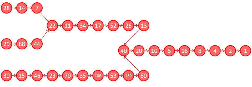
It is remarkable that there is no smooth pattern in the results.  Adjacent integers, such as 26 and 27, can have wildly different stopping lengths, 10 versus 111, respectively, while adjacent pairs can have identical stopping lengths.  Particularly noteworthy is the fact that the integers 28, 29, and 30 all have a stopping length of 18 despite their rather different trajectories:

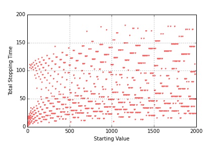
The jerky or random character of the stopping length plot for the first 100 integers transitions into something more akin to patterns within patterns when the number of integers surveyed increases to 2000.

There seem to be overlapping curves asymptotically rising and falling, layered one on top of the other with large regions where they interleave.

Different visualizations reveal different structures.  For example, the stopping times for the first 10000 integers, plotted on a semilog plot

reveal a general triangular shape, whereas the same data shown on a full log-log plot shows

that the values are tending to cluster rather that moving in a unbounded fashion.

This latter observation opened another line of inquiry centered on just how high does the hailstone trajectory go rather than how long does it take for it to land.  A little bit of additional coding to capture the full trajectory for the first 2000 integers reveals that one value, 9232, tends to be hit more often than all the others.

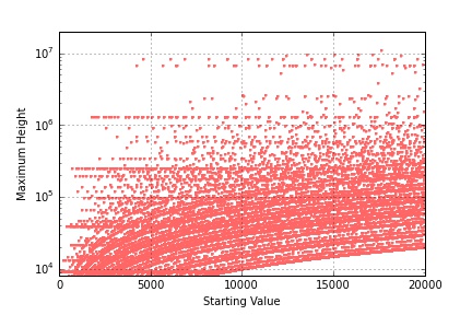
There is a strong line visible just under 10⁴ on the plot and some simple statistics show that 9232 forms 16% of all the highest values in the first 100 integers and about 33.8% for the first 2000.  As the integer range increases to 20000, additional horizontal attractors (to coin a term in relation to the Collatz Conjecture) come in, although it is difficult to pick out just how prominent they are due to the business of the plot.

It is interesting to see just how low these horizontal attractors extend.

As this column closes, it is worth repeating that all of this structure comes from a repeated application of the HTPO process for a finite number of times.  The fact that mathematics can’t say whether the process will stop for arbitrary integers is astonishing and speaks to many of the basic complexities that arise in proof and logic when the repeated operations are involved.  It seems that if Socrates were alive and playing with the Collatz Conjecture he might be inclined to point out that the only wisdom is knowing that we don’t know very much.

The jury is in!  The weight of science has been thrown down on yet another study and now we can all safely rest at night.  We can all look our dentists right in the eye (or should it be mouth?) when he asks have we flossed and we can say “Nope, science says we don’t need to!”

But it is worth asking just why is everyone sure that this is the right thing to do?  Haven’t scientific studies been wrong before?  Wasn’t there science behind the recommendation to floss? Just how long will it be until a new study overturns the old one?  And is it really true flossing has no benefit (outside the profits for the manufacturers)?

Let me take a stab at addressing the first questions immediately and deferring the benefits of flossing until later.

Perhaps the best place to start is by discussing a thought-provoking article entitled Scientific Regress from the May 2016 edition of First Things.  In that piece, William A. Wilson, a software engineer, gives a nice summary and analysis of the state of modern science.  Not the state of its discoveries or knowledge base but the state of what it knows about itself and how it knows what it knows to be true.  In other words, Wilson gives a meta-analysis of the state of the scientific method and its corresponding epistemology.

Of course, the central notion to any of the scientific enterprises is the idea that what happens in the hear-and-now is applicable to the there-and-then.  Without that basic premise, science would nothing more than a set of anecdotes starting with “I swear that I witnessed…”.  It is vital that scientific claims are verifiable.  Repeating an experiment, which should be done often, should give rise to the same results and the same conclusions.  After all, that is the underlying mechanism by which scientific discoveries become technological breakthroughs.  Think what would happen if the original experiment that established the proof-of-concept of the solid state transistor were a one-off.  Goodbye cellphone, household computers, the internet, inexpensive televisions and radios, and hosts of other modern-day goodies.

And yet, the picture that Wilson paints about modern scientific explorations shows a system that is seriously flawed.  He cites the efforts of the Open Science Collaboration (OSC) that tried to replicate 100 published psychology experiments taken from three of the most prestigious journals of the field.  (I’ll have occasion to revisit the notion of prestigious a bit later).

According to the article, OSC found that, in 65 cases, they could not replicate the positive results that were reported in these so-called scientific studies.  In addition, they found that a bulk of the remaining 35 cases were marginal in that their positive results were not nearly as statistically significant as first claimed.

And while other disciplines are not plagued with irreproducibility of this magnitude, there are still many cases where the results of given experiments can’t be corroborated by other groups.

So what is behind this lack of reproducibility? According to Wilson, the answer lies in one of two areas.

First is the possibility that there is a set of confounding variables in the experiment – conditions that need to be controlled but are not recognized as such. For example, if temperature were important in a study of perceptual psychology but was never imagined to be so then the study authors may not report the temperature and therefore their experiment would not be exactly reproduced.  This explanation would be one-part blessing and one-part curse as the presence of such an effect would reveal layers of reality unknown to this point but would make it hard to ever replicate an experiment.  Of course, this kind of thing happens, but to occur with a frequency high enough to explain the OSC results strains credulity.

The second, and more likely reason, is that the original conclusions of the study are simply wrong.  Three possibilities here; what I will call statistical false alarms, group think (what Bacon & Bacon call either Authority or Idols of the Theater), and downright fakery.

The most reassuring one is the statistical false alarms.  There is a nice Bayesian argument that Wilson attributes to John Ioannidis that argues that many scientific studies must be wrong.  The argument goes something like this.  Suppose you have a gem detector that has an accuracy of 95%, which means that if you know it is hovering over a gem it will alert the user positively most of the time and, conversely, if it is hovering over a piece of glass it will not react most of the time.  Armed with this good detector, you then journey out to a field filled with pieces of glass and an occasional gem dropped into the mix.  Since you don’t know which is which and the population of the gems within the greater population of useless baubles is very small, the actual probability of getting a false alarm can be very high.  Details on this kind of argument can be found in an earlier column on Bayesian analysis.  Now consider the gem or useless bauble as a positive scientific discovery or null result, respectively, and the usual machinery of statistical inference to a 95% confidence as the gem detector and you are left to conclude that the possibilities of new discoveries reported in a study bearing up under scrutiny are rather low.

But isn’t this how science feels its way forward?  Isn’t this how we progress?  The answer to these queries is actually a guarded yes.  Our tolerance to being wrong shouldn’t blind us to wrong-doing.  Some of that wrong-doing is subtle and often due to the perverse incentives that we, as a society, has heaped on the scientific enterprise.

Consider the possibility of group think in research.  Positive results receive huge press releases, the promise of fame and fortune, and a huge boost to the intellectual pride.  Articles based on ‘breakthroughs’ aim for large impact factors and all but guarantee tenured positions and speaking circuits. Negative results, often far more important in the scheme of things, are judged to be not worth reporting.  This despite the fact that as Edison famously said about ‘failure’:

Far worse than this institutionalized self-delusion is the case of outright fakery.  As the recent spate of scandals indicate, it is all too common – and not just in the soft sciences.  It is standard to see complaints of plagiarism in the physical sciences (especially from India and China).  Reports abound of authors gaming of the peer-review system by creating aliases for themselves that give them the ability to vet their own articles.

Far worse than any of these offenses is the downright cheating that is becoming all-too common.  There have been amazing examples of the wool being pulled over the collective eyes of peer review.  One of my favorites is narrated in the book Plastic Fantastic, by Eugenie Samuel, which narrates the flummery of one Jans Hendrik Schön a German physicist who became a famous figure in condensed matter physics with his breakthrough results.  He was given two prestigious awards and published in the prestigious journals of Science and Nature (there is that adjective again) before the house of cards came tumbling down when it was determine that he hoodwinked ‘smart’ people for years with amazing but made-up results.  Papers were retracted from many prestigious journals, proving that prestige is more perception than anything else.  Schön’s story is hardly an isolated case and some simple searches can find lots of examples of academic foul play.  There have always been cheats in science but the current system encourages it to a degree never seen before – after all there is big money in and power in science.

So what to do when a new study comes out?  For the most part, take it with a grain of salt, especially if it is predominantly populated by statistical analysis using hypothesis testing with no clear physical mechanism to explain the results.  As for flossing – well I will continue to do it (even though I would love to stop).  The reason being that I have actually experimented with flossing and not flossing and have found that my mouth feels better, I breathe better, and my teeth have fewer complaints (pain, cavities, etc.) for the dentist.  I suspect that the reason that my results are in conflict with this study is that all of human kind can’t be summarized by a ‘representative sample’ and that something about me, whether it is nature or nurture, sets into one of those small populations that Bayesian analysis warns us about.

One of the most remarkable aspects of the human mind is its ability to work with, through imagination and insight, concepts that can’t be worked with in the material world. Nowhere is this more profoundly applied than in the synthesis of human knowledge dealing with the concept of infinity in modern mathematics.

The idea of infinity is the concept of an inexhaustible process that is imagined to be repeated as many times as desired. It is truly amazing that the human mind can abstract what would happen in a particular set of circumstances that can never be realized in the physical world.

Perhaps no scenario illustrates the simple way that insight, imagination, and intuition can be harnessed to deal with infinity than the farmer’s problem.

I must confess that while the particulars of the farmer’s problem presented below are my own, the basic framework came from a popular book on mathematics. Unfortunately, I don’t recall where I found this illustration of the power of infinity so many years ago and so I can only apologize to my source for my forgetfulness and ignorance.

The farmer’s problem can be framed as follows. Suppose that a farmer and his family – his wife and two children – decide to relocate to an off-world colony somewhere in a distant star system. Since space travel limits the amount of stuff that can be transported, our farmer – let’s call him Farmer Lister – wants to be as economical as possible. In particular, he would like to take the minimum amount of grain necessary to get his farm producing the food he and his family needs. Taking more than needed deprives them of space to take other needed resources, like farm equipment, first-aid supplies or the like.

Agricultural reports indicate that the soil on the colony world is conducive to growing wheat, and that a high-yield wheat that produces 3 bushels at harvest for each bushel planted is the optimal choice, based on soil chemistry and climate. Each colonist family brings the essential supplies to get the farm started as well as rations for the first year as the crop grows. At harvest, Farmer Lister needs to have a crop of 3 bushels in order to feed his family in the next year. The question is, then, how much wheat should he pack?

Let’s try out a couple of scenarios.

First suppose that he packs 1 bushel of wheat. During year 1 things are fine as the family plants the first bushel and eats the rations while the crop grows. At harvest, they get 3 bushels of wheat which will support them during year 2 but with nothing left over to plant for subsequent years.

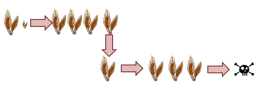
Next suppose that he packs 1+1/3 bushel of wheat, which he plants during year 1. The 1 bushel of wheat produces the 3 bushels his family needs to survive year 2 and the 1/3 bushel produces an extra bushel of wheat for planting in year 2. The survival needs of year 3 are assured but tragically that is where the process stops since the 1 bushel produces only enough for food during year 3 and the Lister family dies of starvation after that.

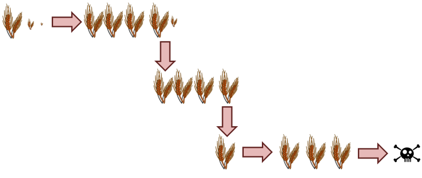
Finally, consider what happens if he adds an additional 1/9 bushel. During year 1 he plants 1 + 1/3 + 1/9 bushels and gets 3 + 1 + 1/3 bushels at harvest. During year 2, his family eats the 3 bushels and plants the 1 + 1/3 bushels for the future. At harvest, the crop yields 3 + 1 bushels. During year 3 his family eats the 3 bushels and plants the 1. At harvest, this last crop yields the 3 bushels they need to eat during year 4 but they get no further.

Clearly he is on the right track but needs to augment the initial supply by a power of 1/3 for each additional year (1/81 to have something to plant in year 4, 1/243 for year 5, and so on). In short Farmer Lister has to figure out how to turn the infinite sum of

\[ 1 + \sum_{n=1}^{\infty} \frac{1}{3^n} \]

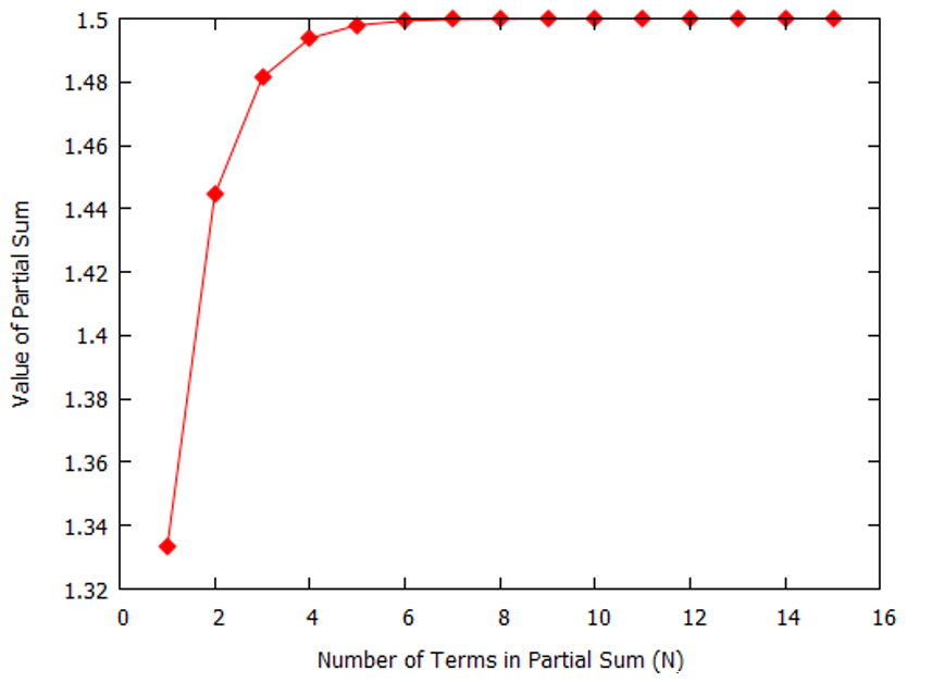
into something he can specify in terms of the goods manifest. Knowing some calculus, he tries graphing the partial sum as a function of $n$ and finds that the partial sums seem to quickly converge to the value of 1+1/2.

Encouraged by this result, he examines what happens if he takes 1+1/2 = 3/2 bushels. During the first year he plants 1+1/2 bushels and gets a final crop yield of 3 + 3/2 bushels. His family now has 3 bushels to eat and 1+1/2 bushels to plant. Thus the process is self-sustaining and he concludes that the infinite sum has a finite value

\[ \sum_{n=1}^{\infty} \frac{1}{3^n} = \frac{1}{2} \; . \]

It is worth noting that Farmer Lister was able to imagine crowing crops indefinitely, even though he can’t actually do that, and was able to have insight into how an infinite number of things combine to form something finite. This is the power of the human intellect and the magic of the process of growing food.

Arguing about cause and effect is a difficult enterprise even in the best of circumstances.  Rarely is it as clean, or as boring, as introductory texts on logic make it out to be.  Examples of simple cause and effect – it is raining and therefore the ground is getting wet – are neither controversial nor are they fun.  Most everyone agrees on the matter and that’s that.  But arguments over new things undiscovered or unseen are one of the best things going.  Who isn’t thrilled by the prospect of figuring something out that none else have done?

Interestingly enough, almost all of us use standard methods for arguing from effect to cause.  Most likely, we’ve all learned these methods by first watching others apply them and then by next jumping into the game and trying out the methods ourselves.  As will be discussed in more detail below, these methods worm themselves into almost every aspect of life; often without our notice.  They form the backbone of most editorials, advertisements, and dinner-table arguments.  And despite their anonymity, they do have a name:  Mill’s Methods.

First codified by John Stuart Mill in his book A System of Logic (1843), these methods, which no doubt date back to antiquity, go by the obscure names of:

• Method of Agreement
• Method of Difference
• Joint Method
• Method of Concomitant Variation
• Method of Residues

As unfamiliar as these terms may be to the ear, their use and application is familiar to the thinking of anyone who has ever tried to figure out what food at dinner last night didn’t agree with them or some similar scenario.  Indeed, many of the examples presented in the community deal with food and indigestion.  (In fact, application of Mill’s Methods to epidemiology is the core component of the TV show House).

Not wanting to dwell on food related illness (since it is done to death in the literature), I propose illustrating the methods using a more interesting question faced by parents and teachers across the country:  what factors contribute to good grades.

Consider a group of 10 students from a local school.  After circulating a questionnaire, their teacher compiles a table listing various activities they pursued and the study method they used (written homework or online quizzes).  The teacher wants to see what caused half the students to pass where the other half failed and so he looks for a factor that is both necessary and sufficient to explain why the first group passed.  He suspects that those students who play video games have been poisoned and that students who avoid this digital scourge are the ones that pass.  But being a man of integrity he decides to pursue the answer with an open mind.  To do this he employs Mill’s Methods in succession.

To apply the Method of Agreement, he looks to see what features all the passing students have in common.  He starts by looking at a subset group composed of Amy, Carl and Walter.

He notices that these 3 students have nothing in common in terms of their recreational pursuits, they don’t play the same musical instrument (in fact Amy doesn’t play any), that that they don’t all engage in the same exercise.  But all three of them were taught using the same technique of written homework.  He concludes that there is very likely possibility that written homework is the cause of their success in the class.

To apply the Method of Difference, he then looks for a pair of students, one who has passed and one who has failed, that have almost everything in common.  Any difference between them being a strong indication that it is the cause of success/failure.  He finds such a pair in Ben and Stacey.

Both of them enjoy blogging, play guitar, and exercise by running.  The difference between them seems to be that Stacey was required to do written homework while Ben was required to do online quizzes.  He concludes that there is a very strong possibility that written homework leads to good grades.

The Joint Method marries the two approaches together looking for support that this one factor, the teaching technique, is the primary cause of classroom success.  To this end, our teacher combines all the students into the following table

and he notices that in each case, the only factor that correlates with passing or failing, is written homework or online quizzes, respectively.  Despite his preconception that video games were dangerous he finds that two of the three students (Amy and Vanda) who play actually passed the course.

The final two of Mill’s Methods deal with matters of degree.  They help to answer how much written homework really helps and if there is another factor that might contribute to success.  To this end the teacher modifies the table to list the hours each student spends completing their written homework and their GPA.

In the case of the Method of Concomitant Variation, the teacher notices that in there is a strong correlation between the number of hours of homework each week and the student’s GPA.  Vanda does the least amount of homework each week and she has the lowest GPA.  Carl and Stacey are in the middle in terms of time invested in homework and so is their GPA.  And finally, Amy and Walter have the highest time spent on homework and the highest GPA.  This behavior is a strong indication that requiring students to complete written homework causes students to have high GPAs.

The Method of Residues helps to point towards additional factors that have not been considered but which contribute to the cause and effect relationship.  In the case of the two top performing students, the teacher notices that although Amy spends the greatest amount of time on homework each week she doesn’t have the highest GPA.  Of course, this minor difference between her and Walter might be explained in many ways (e.g. her courses are harder).  But let’s suppose that the table exhaustively lists all the relevant attributes and that Walter and Amy are in the same class in elementary school so that they see all the same material and are assigned the same homework.  Our teacher might be inclined to conclude that either playing a musical instrument or exercising might be the cause of the remaining difference.  This method can also be applied to the situation were the differences are a matter of quality rather than quantity.

One of the most famous examples of the application of the Method of Residues was to the motion of the planet Mercury.  After all the known contributions of Mercury’s orbit had been accounted by astronomers of the late 1800s there was still a remaining 53 arcseconds/century of precession that could be ascribed to any particular cause.  This difference, though small, helped to spur Einstein to create the theory of General Relativity.

While the discussion above was both illustrating and interesting it is hardly the only nor primary application of Mill’s Methods.  As Prof. Dave Beisecker points out on his discussion, Mill’s Methods are used in all sorts of persuasive arguments about products, policies, and the like.  I would encourage the reader to visit his page as some of his examples are both educational and laugh-out-loud funny.  Consider this gem used to illustrate how the Method of Difference is used in advertising

Of course real life is never so clear cut as the contrived examples seem to imply.  But that’s what makes it so fun.  Putting one’s skill to the test to find what causes what can lead to amazing discoveries and brings out the best in us.