
Images, Representations, and Programming
It’s an old idea. Someone you know holds up a photograph depicting something familiar, say a beautiful car, maybe a Corvette, and asks you “what this?”. You answer, “it’s a Corvette,” and are greeted with the cheeky response, “No! silly, it’s a picture.”
This simple joke, while annoying, makes an important philosophical point about keeping a clear distinction between the image of a thing and the thing itself. As important as this distinction is for basic reasoning and logic, it is much more important to keep it straight in the practice of mathematics and computing – particularly in the study of vectors.
Formally, a vector is any kind of object that belongs to a class of like objects that all ‘obey’ a set of rules that define how they combine to form new objects also in the same class. For simplicity, a vector will be denoted in underlined, bold face but, as will discussed below, there are other common ways to denote the vectors, all of which suffer from ‘Corvette-problem’ above. The set of combination rules are:
- There is a combination rule ‘+’ such that U + V is a vector if U, V are vectors
- U + V = V + U (order doesn’t matter)
- U + (V + W) = (U + V) + W (the combination rule is associative)
- 0 + U = U + 0 = U (there is a zero vector)
- U + (-U) = 0 (there is a way to add up vectors to get a zero one)
- There is a scaling rule such that the product kU is a vector, (k is an ordinary complex number)
- k(U + V) = kU + kV
- (k+l)U = kU + lU (where k & l are ordinary complex numbers)
- k(lU) = (kl)U
- 1U = U
Some purist out there may object and point out that only occasionally does an author actually enumerate all 10 items above separately (even though such a purist will concede that all 10 must be there in some form or another). The purist may also go on to say that some authors prefer 0U = 0 to rule #5. But none of these details are particularly important.
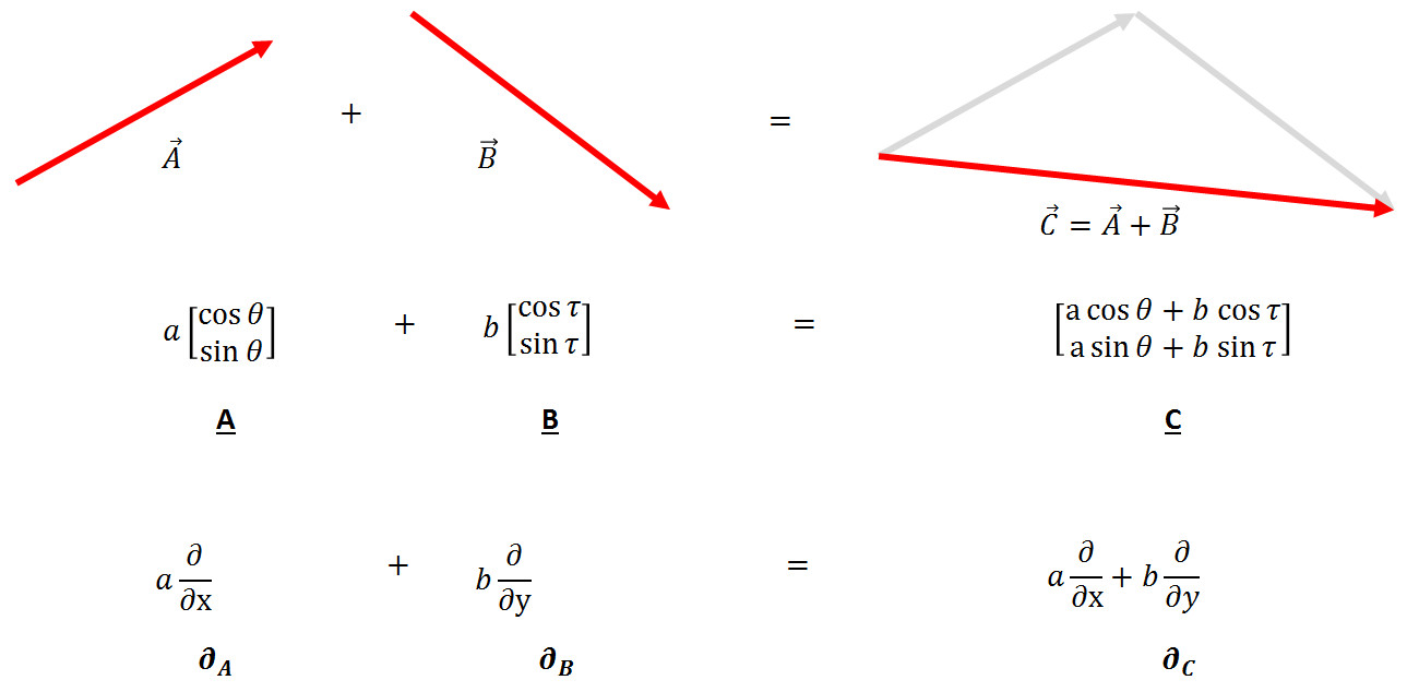
What is important is that the rules are abstract and simple. They apply equally well to vectors defined as a directed arrows as they do to vectors defined as column arrays of numbers as they do to vectors defined in terms of partial derivatives. They apply equally well to vectors that we can observe and touch, for example pulls and pushes on an object, as they do to those that live in an abstract space like column arrays or partial derivatives, whose sole existence is built from ideas in the mind and symbols on the page.
As the study of vectors deepened, several clarifying points made computation with them very simple. The most powerful, and hence most dangerous, realization is the point that an arbitrary vector can be decomposed in terms of primitive vectors, usually referred to as basis vectors. This realization, which arguably finds its crystallization in the work of Descartes, reduces the infinity of possibilities into a manageable number of chunks and is the driving force between the 10 rules listed above.
The manageable chunks consist of a set of basic vectors whose number equals the number of dimensions in the space (1 for a line, 2 for a plane, 3 for a volume, and so on) and a list of the numbers whose length also equals the number of dimensions.
And here is the first of the traps. Once the basis vectors are agreed-upon and understood, they can be pushed to the back and the list (called a list of components) can be manipulated without much additional thought. The list becomes a stand-in for the original object in analogy for the way that the image of the car becomes a stand-in for the car itself. The list is now a representation of the original object.
This blurring between the original object and its representation becomes even more fuzzy with some additional reflection. A list is also a valid choice as an original object in the vector space since it also obeys the 10 rules (with the appropriate definition of ‘+’ and ‘x’). To show how strange this is in the physical world, consider the possibility of getting into the picture of the car, kicking over its motor, and taking it for a spin.
It’s no wonder that otherwise well-trained and intelligent people get hung up over vectors and their manipulations each and every day. Functionally, every object shown in the figure above is equivalent to a list of numbers.
Now suppose that one wanted to represent these abstract objects in a computer language. Well, as long as one was careful, one could actually exploit these ambiguities and simply say that the list will always be the representation. This is actually what most, if not all, languages do, though they differ in the terminology, with many choosing array, some choose vector, and others stay with list.
Of course, most users aren’t careful about maintaining that distinction and, I suppose, most aren’t even really conscious of it. But one hopes that at least the language creators do.
In most cases, this hope is realized. Many languages make the distinction between a heterogeneous list (not a vector) and a homogeneous list (which is, or at least can be, a vector). Some languages, like those underlying the computer algebra system Maple, use the word vector to connote a special kind of list. However, sadly, sometimes a language gets befuddled and either loses these distinctions or creates ones where none exist.
An example of the later problem comes from the numpy/scipy family of packages used in the Python programming language. To properly discuss this minor defect in what is really a great set of packages, I need to add one more ingredient that adds a few more ingredients to the vector space turning it into a metric space.
In a metric space, there is added to the original 10 rules an additional notion of the length of a vector. A new combination rule, usually denoted with a dot ‘.’, allows for two vectors to be combined to produce not another vector but a number, specifying how much of the length of one of the two lies along the other. This combination is defined such that A.B = B.A and that A.A is the square of the length of A. This combination rule is called variously as a dot product, an inner product, or a scalar product.
Once defined, another operation can be derived from these 11 rules. This operation, called the cross product, mixes the components from various places in the list to get new components. It depends on the dot product to bring meaning to the idea of having the component from one dimension multiplying the component from another dimension and, like the dot product, actually results in an object that doesn’t (properly) belong in the vector space. In other words, both the dot and the cross products take two vectors and produce something different.
In addition, both rules belong to the space itself since they both apply to any two pairs of vectors. Unfortunately, the numpy/scipy team missed this concept entirely.
In numpy, the vector space as a whole can be thought of as being represented by the family of functions that make up numpy proper. These functions include the function ‘array’ for making a new array and the function ‘cross’ for taking the cross product. Strangely, the function ‘dot’ is not found in the collection of numpy functions but rather is a member function of the ‘array’ object itself. A minor flaw in a really fine set of packages but a solid proof that it isn’t always easy to the tell the image from the thing.