A Symbolic Experiment – Part 6: Elementary Term Rewriting
After many months of build-up, we are now in a position to begin methodically exploring how to modify Sympy expression trees that we have defined earlier. Since Sympy expressions are, by design, immutable, it is important to understand that when terms like ‘modify’, ‘change’, ‘substitute’, ‘replace’ and other synonyms are used they are short hands for the more precise but far more wordy phrases like ‘making a new expression whose structure is a modified version of an older expression’ or ‘making a new expression that is based on an older expression but for which certain subexpressions have been replaced’, and so on. While the shorted phrases are easier to deal with it is vital that we don’t forget that they aren’t to be taken literally.
Methods for making changes to an expression tree can be grouped into two broad categories: 1) by-hand methods and 2) built-in methods.
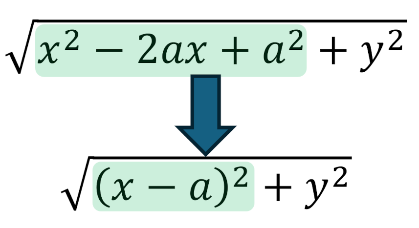
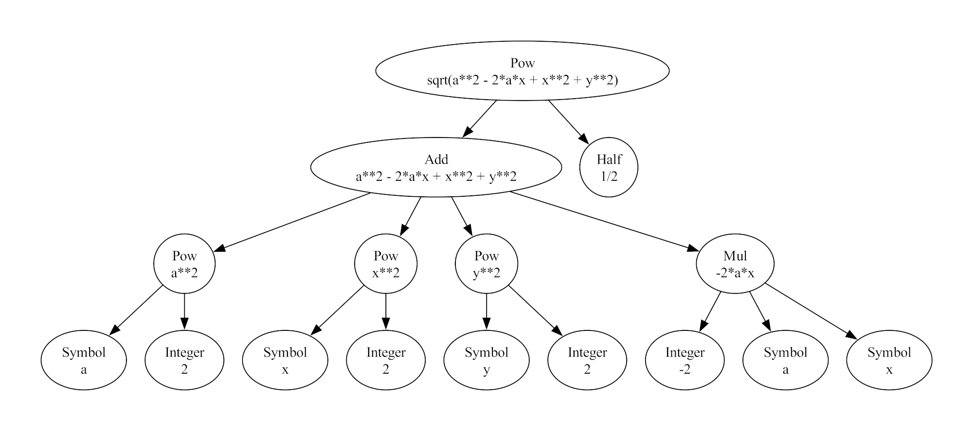
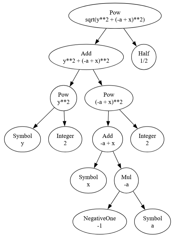
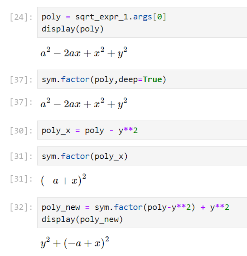
An example of a by-hand method was featured in an earlier post about factoring where a small function using .has, .as_ordered_terms, and .factor was used to factor the, by now very familiar, test case of
\[ x^2 – 2ax + a^2 + y^2 \rightarrow (x-a)^2 + y^2 \; .\]
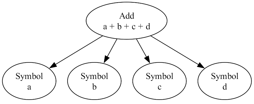
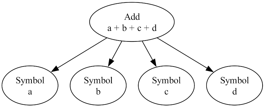
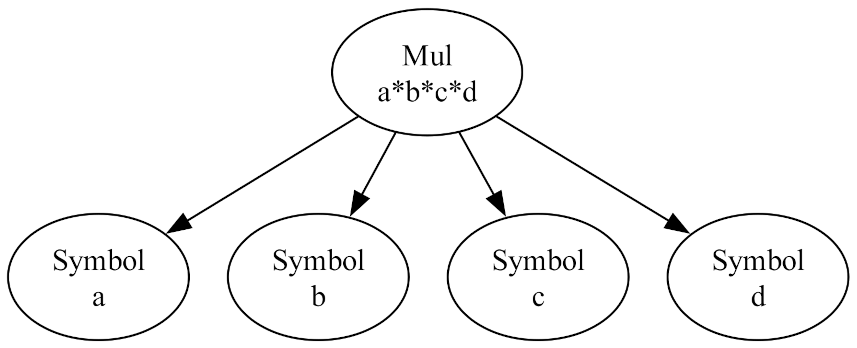
The use of .has(a,x) (see last post) allows the relevant terms to be separated from the polynomial without needing to ‘see’ them or ‘spell out’ what they are. The function .as_ordered_terms was used to separate the top level of the Add function. Note that for other types of expressions, other choices, like .as_ordered_factors (for Mul) and args, may be needed, with args being the most generic of the lot. The key point being that the tree was ‘broken down’ into smaller pieces, some of which were amenable to the kinds of simplification functions discussed in a previous post.
There are three often used functions in the second category of built-in methods. On these points, I received an excellent high-level summary from Oscar Benjamin, who is a Sympy developer. I will draw on this summary for what follows with two caveats: first, these methods are nuanced and complex, so I won’t be able to fill in as ably as one of the developers can and, second, any mistakes are solely a consequence of my ignorance.
The three methods are .xreplace, .subs, and .replace, given in order of what seems to be best described as generality and complexity. That is to say that Oscar Benjamin has described them as:
The xreplace function is the fastest and simplest. The replace function is the most flexible. The subs function is the slowest and is the only one that applies any semantic meaning to the substitution.
The following table summarizes their usage.
| Method | Usage | Comment |
| .xreplace | expr.xreplace({o1:n1, o2:n2, …}) | Purely structural replacement which identifies a exact subexpression to be replaced (hence the ‘x’ in xreplace). |
| .subs | expr.sub({o1:n1, o2:n2, …}) | Mostly structural replacement but some mathematical equivalence is used in simplify terms. |
| .replace | expr.replace(old_pattern,new_pattern) | Purely structural replacement which uses a generic pattern to replace all subexpressions that match) |
Note: {o1:n1, o2:n2, …} is a dictionary specifying how old expressions (o1, o2, etc.) are to be replaced by new terms (n1, n2, etc.).
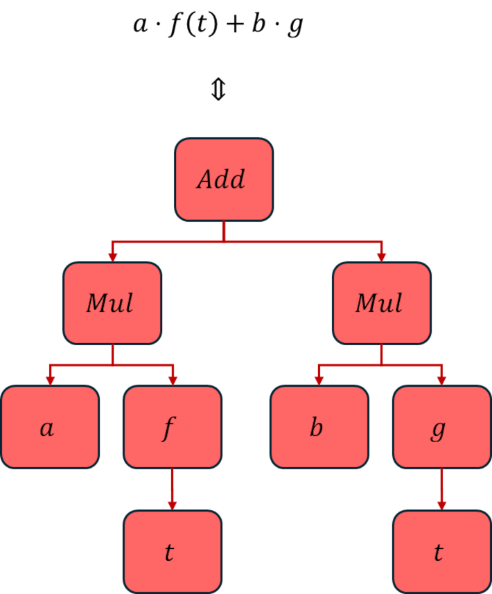
In order to illustrate the differences between these methods, we’ll start with the master expression
\[ Q = a + x + 2 x^2 + 3 x^3 + 4 x^4 + 5 \cos(x) + \\ 6 \cos(x^2) + 7 \cos^2 (x) + 8 \cos(b) + 9 e^{-x^2} \; .\]
We’ll look at all three methods under two term-rewriting rules:
- Rule 1: $x^2 \rightarrow y$
- Rule 2: $\cos(x) \rightarrow \sin(x)$
Rule 1: $x^2 \rightarrow y$
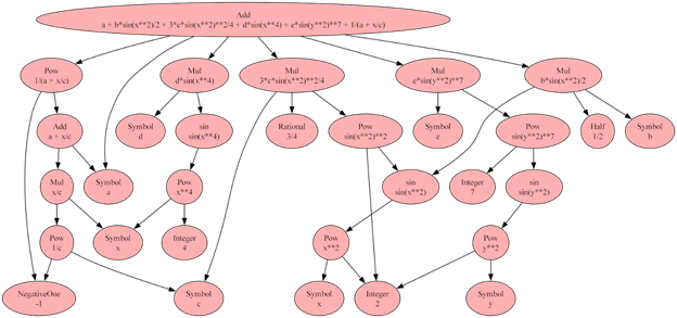
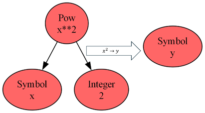
Under the action of .xreplace $Q$ becomes
\[ Q \xrightarrow{x^2 \rightarrow y} a + x + 2 y + 3 x^3 + 4 x^4 + 5 \cos(x) \\ + 6\cos(y) + 7 \cos^2(x) + 8 \cos(b) + 9 e^{-y} \; ,\]
showing that .xreplace simply went through $Q$’s tree structure and structural rewrote sub-trees as shown in the following figure.
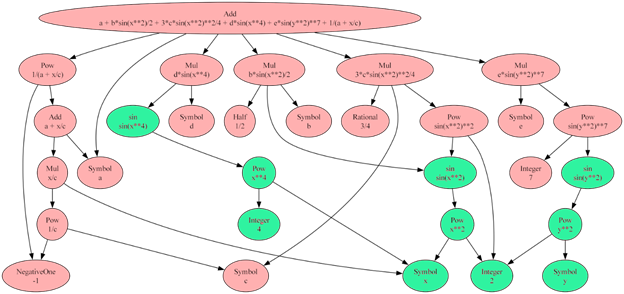
Under the action of .subs $Q$ changes more, becoming:
\[ Q \xrightarrow{x^2 \rightarrow y} a + x + 2 y + 3 x^3 + 4 y^2 + 5 \cos(x) + \\ 6\cos(y) + 7 \cos^2(x) + 8 \cos(b) + 9e^{-y} \; .\]
Note that .subs ‘understood’ that $x^2 \rightarrow y$ properly, and without assumptions, means that $x^4 \rightarrow y^2$. Odd powers of $x$ remain unchanged since .subs doesn’t know enough to invert the replacement since it would have to choose between $x \rightarrow +\sqrt{y}$ and $x \rightarrow -\sqrt{y}$.
Finally, under the action of .replace, $Q$ yields
\[ Q \xrightarrow{x^2 \rightarrow y} a + x + 2 y + 3 x^3 + 4 x^4 + 5 \cos(x) + \\ 6\cos(y) + 7 \cos^2(x) + 8 \cos(b) + 9 e^{-y} \; ,\]
which is exactly identical to what resulted from the application of .xreplace.
Rule 2 $\cos(x) \rightarrow \sin(x)$
Under the application of .xreplace, $Q$ becomes
\[ Q \xrightarrow{\cos(x) \rightarrow \sin(x)} a + x + 2 x^2 + 3 x^3 + 4 x^4 + 5 \sin(x) + \\ 6\cos(x^2) + 7 \sin^2(x) + 8 \cos(b) + 9 e^{-x^2} \; , \]
again, as in the example for Rule 1, .xreplace only makes a structural change/rewrite for only those subexpressions that, in a tree-sense, exactly match the old subexpression.
The application of .subs gives identical expressions for $Q$, as does a naïve use of .replace. However, a much more interesting example using .replace involves using Sympy’s ‘Wild’ symbol. The following snippet of the Jupyter notebook
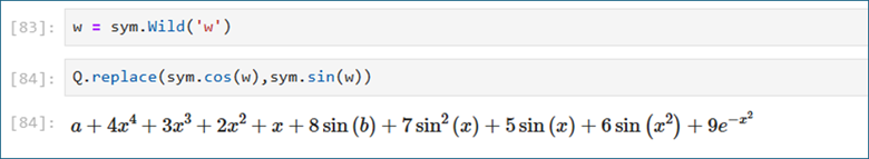
shows how .replace can substitute the sym.cos node with a sym.sin node without affecting the leaves and branches of the tree underneath. That’s why every instance of $\cos$ changes to $\sin$ regardless of whether the argument was $b$, $x$, or $x^2$.
Final Thoughts
There are a number of variations and nuances that haven’t been covered above but I believe that with the material provided there is enough structure that the Sympy documentation is consumable and a person who understands the material so far should be able to reach the manipulations they want with only some limited trial-and-error. That said there are two nuances that are worth noting. First, .subs is aware of what Sympy calls bound variables. Bound variables are those that appear, for example, as part of a sum or integral; .subs will not allow them to be rewritten while .xreplace will – again because .subs has some notion of mathematical semantics whereas .xreplace is simply for changing the tree regardless of syntax. The other is that .replace can take functions as arguments so that complex selection of subexpressions can be done. It is that latter functionality that we will try to use as we finally return to our main goal of having a Fourier transform rewriting system.