
Chaos Game Part 1 – The Basics
As is typical of many of the best things in life, discovery of this month’s topic involved quite a bit of serendipity. It all started with a search for a quick reminder on how to solve a numerical set of coupled ODEs using scipy/Python and it ended with the results seen here on the chaos game.
Since it is possible that the reader is unfamiliar with this term (as was the author), a quick introduction is warranted. In short, the chaos game is a random method for producing a deterministic fractal shape. Its operation is in sharp contrast to the more traditional way of drawing a fractal deterministically by hand in that the chaos game teases out the fractal’s attractor by iteratively applying a set of affine transformations, each chosen randomly, to a series of points starting with a randomly chosen initial point.
Mathematically, the chaos game falls under the broader heading of an Iterated Function System (IFS) where the ith point in the plane $q_i$ is given by
\[ q_i = M^{(p)} q_{i-1} + f^{(p)} \; \]
or, in terms of arrays
\[ \left[ \begin{array}{c} x_i \\ y_i \end{array} \right] = \left[ \begin{array}{cc} a^{(p)} & b^{(p)} \\ c^{(p)} & d^{(p)} \end{array} \right] \left[ \begin{array}{c} x_{i-1} \\ y_{i-1} \end{array} \right] + \left[ \begin{array}{c} f^{(p)} \\ g^{(p)} \end{array} \right] \; .\]
The index $p$ is an integer to label the various affine transformations available, and is chosen at random at each step according to some pre-defined probability distribution.
Before getting to the Python code, which is easy to implement, it is instructive to compare and contrast the traditional method and the chaos game in generating the well-known Sierpinski Triangle fractal.
The traditional way to draw the Sierpinski Triangle starts with an equilateral triangle.

A similar triangle half in size (or a quarter in area) is removed from the middle of the larger triangle leaving an arrangement of three smaller triangles.

The process can then be applied to these smaller triangles yielding another stage of refinement. This in turn results in a larger set of smaller triangles to which the process can be applied yet again.
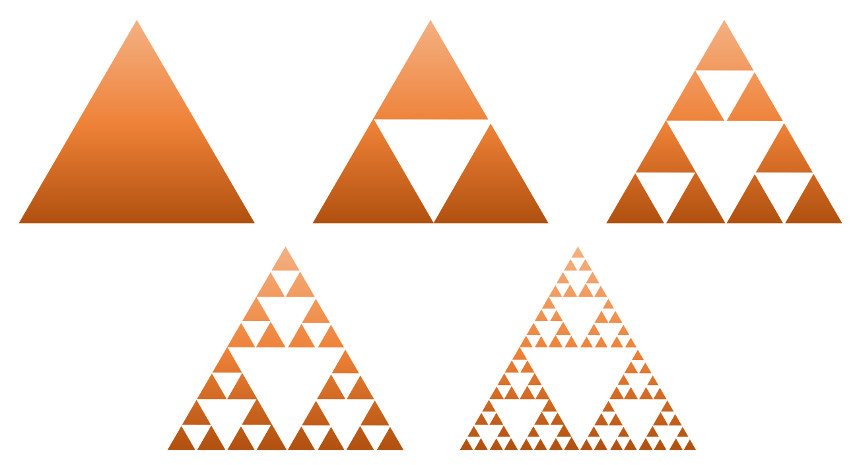
Continuing on indefinitely gives the Sierpinski Triangle in all its glory.
However, there is a fundamental limit on how much can be drawn by hand or by computer, and the amount of work to obtain a successively more exact approximation in level of detail becomes increasingly more immense.
In the chaos game, the programing is much simpler and, due to the random nature of the system, all levels of detail are present simultaneously. Central to the chaos game approach are the three affine transformations:
\[ T1: \left[ \begin{array}{c} x_i \\ y_i \end{array} \right] = \left[ \begin{array}{cc} 0.5 & 0 \\ 0 & 0.5 \end{array} \right] \left[ \begin{array}{c} x_{i-1} \\ y_{i-1} \end{array} \right] + \left[ \begin{array}{c} 1 \\ 1 \end{array} \right] \; ,\]
\[ T2: \left[ \begin{array}{c} x_i \\ y_i \end{array} \right] = \left[ \begin{array}{cc} 0.5 & 0 \\ 0 & 0.5 \end{array} \right] \left[ \begin{array}{c} x_{i-1} \\ y_{i-1} \end{array} \right] + \left[ \begin{array}{c} 1 \\ 50 \end{array} \right] \; , \]
and
\[ T3: \left[ \begin{array}{c} x_i \\ y_i \end{array} \right] = \left[ \begin{array}{cc} 0.5 & 0 \\ 0 & 0.5 \end{array} \right] \left[ \begin{array}{c} x_{i-1} \\ y_{i-1} \end{array} \right] + \left[ \begin{array}{c} 50 \\ 50 \end{array} \right] \; .\]
At each stage of the iteration, one of these transformations is selected with probability 1/3; that is to say that each is equally likely to be selected.
Four basic pieces of code are used in the implementation.
The first is a table that encodes the selection probability and the parameters for each affine transformation used in the game (i.e., each row of the table encodes the likelihood and the numbers associated with $T1$, $T2$, and so on). The table encoding for the Sierpinski Triangle is:
sierpinski_triangle = np.array([[0.33,0.5,0,0,0.5, 1, 1],
                                [0.66,0.5,0,0,0.5, 1,50],
                                [1.00,0.5,0,0,0.5,50,50]])
Second is the Transform iteration function that takes as input the current point, the table describing the game, and a random number simulating the probability at each step.
def Transform(point,table,r):
    x0 = point[0]
    y0 = point[1]

    for i in range(len(table)):
        if r <= table[i,0]:
            N = i
            break

    x = table[N,1]*x0 + table[N,2]*y0 + table[N,5]
    y = table[N,3]*x0 + table[N,4]*y0 + table[N,6]

    return np.array([x,y])
Third is looping code that carries out the chaos game through successive applications. The code, which, for convenience, wasn’t encapsulated in a function, looks like
N     = 100000
shape = np.zeros((N,2))
probs = np.random.random(N)
game  = sierpinski_triangle

for i in range(1,N):
    shape[i,:] = Transform(shape[i-1,:],game,probs[i])
The parameter N sets the number of desired iterations; the numpy array shape pre-allocates the space for the resulting points from the iterations and initializes the starting point to the origin. The probabilities are also precomputed since a call to the numpy (np) random is more quickly performed when in bulk than at each step. The game object points at the particular table encoding the transformations, here the sierpinski_triangle table defined above. The for loop could be done faster using a list comprehension but at the loss of clarity. Since N = 100000 takes less than a second of computation there wasn’t a compelling reason to lose the clarity.
The final step is a plot of the results. The code that performs this is given by
start = 0

fig_shape = plt.figure(figsize=(6,6))
ax_shape  = fig_shape.add_subplot(1,1,1)
ax_shape.scatter(shape[start:,0],shape[start:,1],marker='.',color='k',s=0.01)
ax_shape.axes.set_frame_on(False)
ax_shape.xaxis.set_visible(False)
ax_shape.yaxis.set_visible(False)
The parameter start sets the number of initial points to ignore. This is sometimes useful to suppress the initial stray n points until the game converges to the fractal attractor.
All of these pieces were put together in a Jupyter notebook. The resulting image is
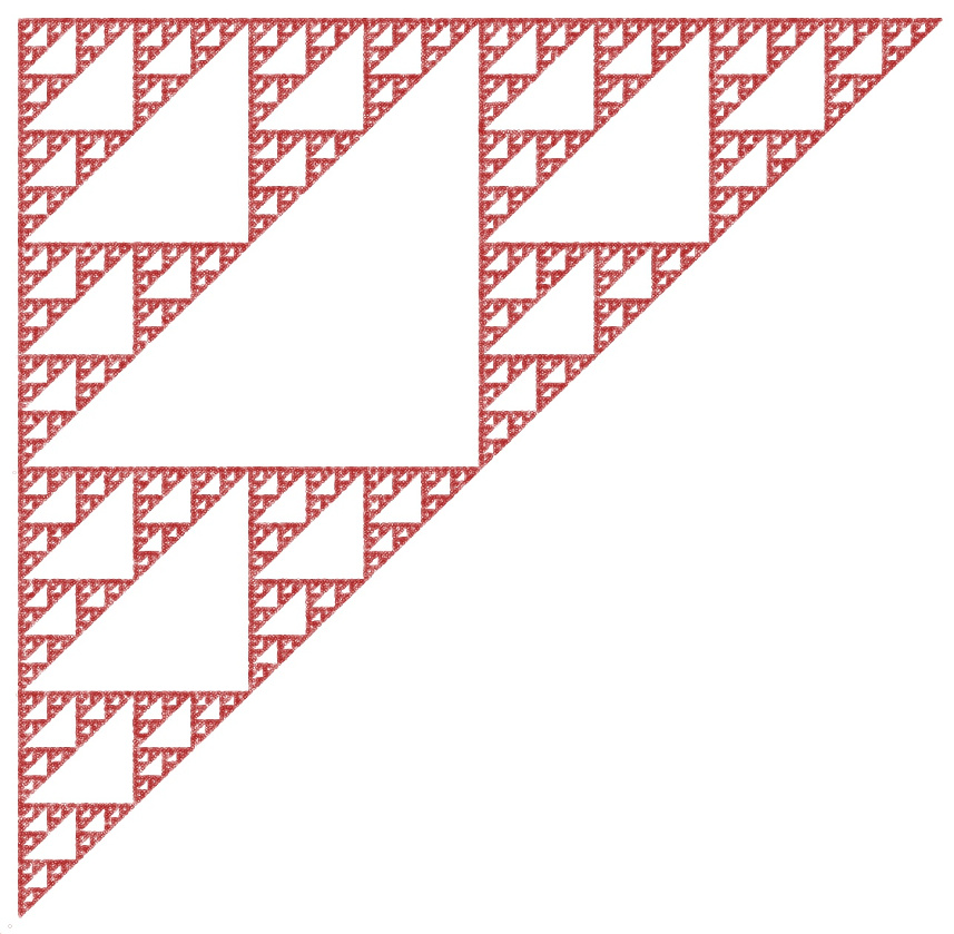
Note that the Sierpinski Triangle is rotated 45 degrees from the more usual ‘artistic’ expression. That minor issue is easily rectified using a simple rotation matrix
c45 = 1.0/np.sqrt(2.0)
s45 = 1.0/np.sqrt(2.0)
A   = np.array([[c45,s45],[-s45,c45]])

new_shape = np.array([A.dot(shape[i,:]) for i in range(len(shape))])
where the parameters c45 and s45 are shorthand for $\cos(45 {}^{\circ}) = 1/\sqrt{2}$ and $\sin(45 {}^{\circ}) = 1/\sqrt{2}$, respectively.
The resulting image is now more aesthetically pleasing.
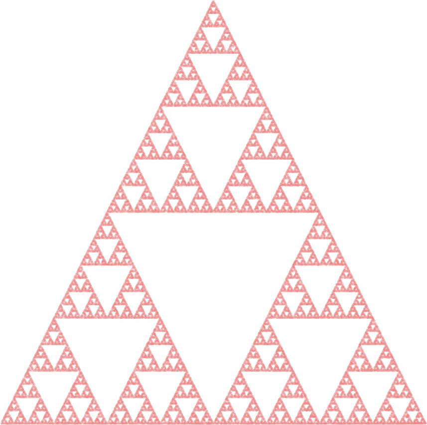
Making it an equilateral triangle is left as an exercise for the reader.
Note that I’ve played with the color scheme freely and inconsistently from image to image. Picking and playing with colors is one of the most fun things about exploring the chaos game.
Future columns will look more closely at the chaos game, why it works the way it does and some of the beautiful images that can be produced.