
Chaos Game Part 2 – How It Works
Last month’s blog introduced the idea of the chaos game, which is a simple and compact computing method for generating deterministic fractals using a Monte Carlo-like random method. The central ingredients of the chaos game are an affine transformation of the plane
\[ \left[ \begin{array}{c} x_i \\ y_i \end{array} \right] = \left[ \begin{array}{cc} a^{(p)} & b^{(p)} \\ c^{(p)} & d^{(p)} \end{array} \right] \left[ \begin{array}{c} x_{i-1} \\ y_{i-1} \end{array} \right] + \left[ \begin{array}{c} f^{(p)} \\ g^{(p)} \end{array} \right] \; , \]
which expresses the current point (labeled by the index i) in terms of the previous point (labeled by the index i-1) in terms of known, fixed parameters $\{a^{(p)}, b^{(p)}, c^{(p)}, d^{(p)}, f^{(p)}, g^{(p)}\}$. The index $p$ is an integer label for the various affine transformations available and is chosen at random at each step, according to some pre-defined probability distribution. For the Sierpinski triangle discussed in the previous post, $p$ can take on the values (1,2,3) each with probability 1/3.
It is convenient to package all the information into a table with each row corresponding to a one of the affine transformations. For the Sierpinski triangle, the table is given by
| Cumulative Probability | a | b | c | d | f | g |
|---|---|---|---|---|---|---|
| 0.33 | 0.5 | 0 | 0 | 0.5 | 1 | 1 |
| 0.66 | 0.5 | 0 | 0 | 0.5 | 1 | 50 |
| 1.00 | 0.5 | 0 | 0 | 0.5 | 50 | 50 |
, which is directly translated into the numpy array
sierpinski_triangle = np.array([[0.33,0.5,0,0,0.5, 1, 1],
                                [0.66,0.5,0,0,0.5, 1,50],
                                [1.00,0.5,0,0,0.5,50,50]])
used for simulation (details in the previous post).
The above material, which is a quick recap of last month’s entry, sets the stage for this post, which focuses on understanding how the structures emerge from such a simple set of rules.
A good starting point for that understanding is the Numberphile video on the chaos game
The presenter, a mathematician by the name of Ben Sparks, starts by showing how the chaos game for the Sierpinski triangle is played by examining single iterations performed by hand. He performs a single iteration by taking the initial point, rolling a six-sided die (yes die is the correct word for the singular – like Sparks that grammatical rule confuses me as well) to randomly pick one of the three vertices, connecting the point to the chosen vertex with a straight line, and then establishing the new point at a distance halfway along that line.
To map this procedure to a mathematical algorithm, start with the situation pictured below.
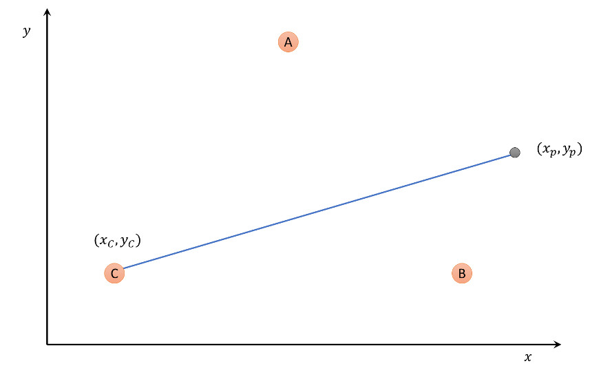
Assuming that vertex C is chosen by random, the line joining the current point to the vertex is given by
\[ \left[\begin{array}{c} x \\ y\end{array}\right] = \left[ \begin{array}{c} x_p \\ y_p \end{array} \right] + \lambda \left[\begin{array}{c} x_C – x_p \\ y_C – y_p\end{array}\right] \; , \]
where the parameter $$\lambda$$ ranges from 0 to 1, with 0 corresponding to the initial point and 1 to vertex C. The point halfway from the initial point to the vertex C has coordinates given by substituting $\lambda = 1/2$ to yield
\[ \left[\begin{array}{c} x_{1/2} \\ y_{1/2}\end{array}\right] = \frac{1}{2}\left[ \begin{array}{c} x_p \\ y_p\end{array}\right] + \frac{1}{2} \left[\begin{array}{c} x_C \\ y_C\end{array}\right] \; . \]
By comparing this formal transformation with the rows of the table, it is obvious that the vertices of the triangle used in the chaos game are: A – (2,2), B – (2,100), C – (100,100). This is nicely confirmed by putting the axes back on the figures and foregoing the aesthetic transformation used last month.
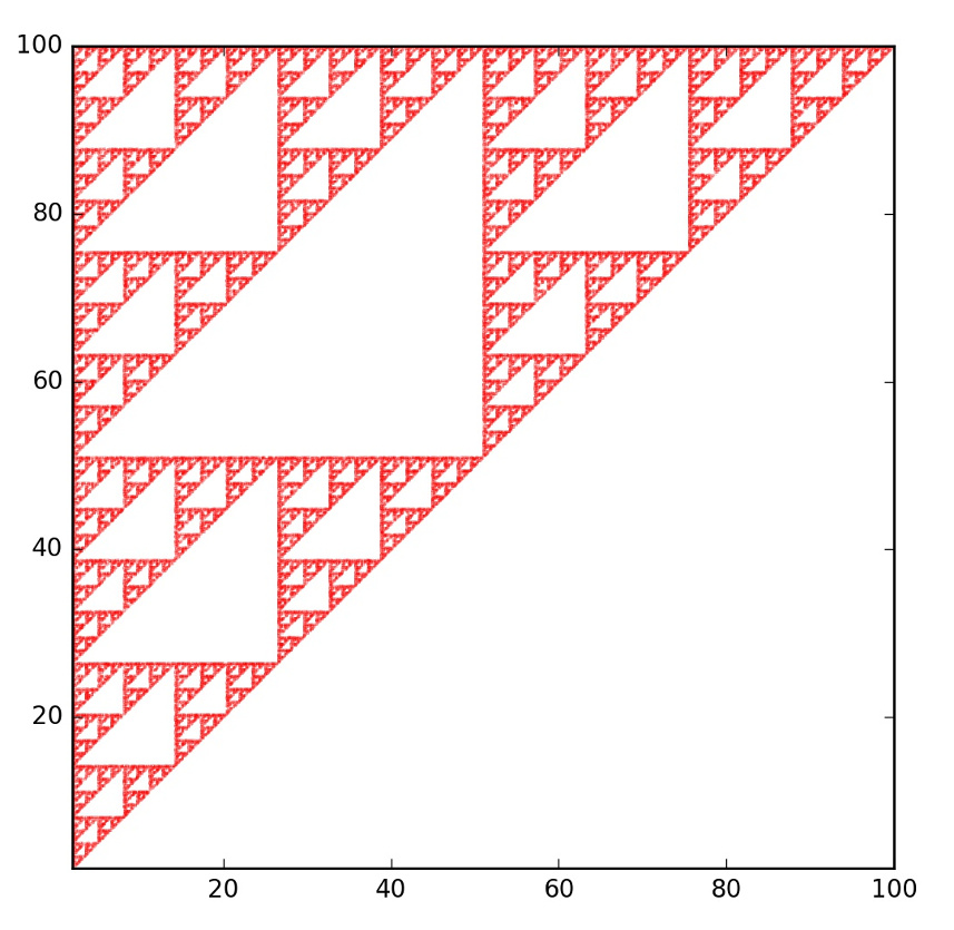
The limits of the figure are [2,100] for the x-axis and y-axis and the triangle fits perfectly into the upper left half.
Further confirmation is obtained by changing the values of $f$ and $g$ for all three affine transformations so that the vertices are now located at: A – (0,0), B – (0,20), C – (20,20). Rerunning the chaos game yields the following fractal
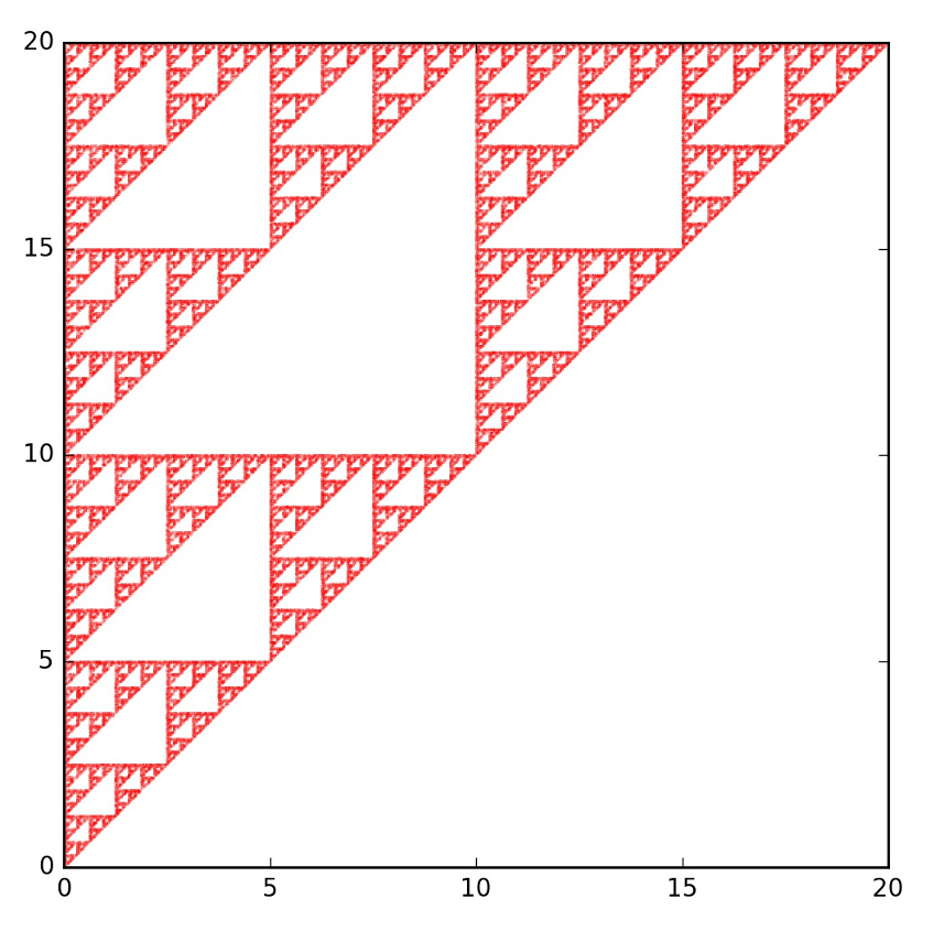
Here the limits on the plot are [0,20] for both the x- and y-axes.
With a firm understanding of what the parameters $f$ and $g$ do, next turn attention to the matrix-portion of the transformation. Referring to the half-way point equation above, the first term on the right-hand side can be recast as
\[ \frac{1}{2} \left[ \begin{array}{c} x_p \\ y_p \end{array} \right] = \left[ \begin{array}{cc} 1/2 & 0 \\ 0 & 1/2 \end{array}\right] \left[\begin{array}{c} x_p \\ y_p\end{array} \right] \; ,\]
thus explaining what the parameters $a$, $b$, $c$, and $d$ describe. For example, to get to point a third of the way along the line connecting the current point to the particular vertex, the table should be changed so that $a = 1/3 = d$ while keeping $b=0=c$.
Finally, the cumulative probabilities can be modified as well to create additional realizations of the game.
Next post will explore some of the various new fractals that can be obtained by fiddling with the matrix component of the affine transformation and the cumulative probabilities as a way of investigating the stability of the game to variations.