
Category Theory Part 1 – An Introduction
Since it is fashionable to start a new year with a new resolution, I thought it might be fun to try something new within the domain of this blog. So, starting this month, the content and approach will be a little different. I’ll be working through Conceptual Mathematics: A first introduction to categories, by F. William Lawvere and Stephen H. Schanuel.
I had picked up this book some time back based on a whim and the promise on the back cover (obviously not quite a wing and a prayer but one improvises). The authors claimed that categories lead to “remarkable unification and simplification of mathematics” and such a bold claim easily caught my attention and sparked my curiosity. Thumbing through the pages made it clear that this work sits as much in the realm of philosophy as it does mathematics and that moved it from a possible purchase to an immediate sale. However, life being life, I only got through the first chapter or so before overriding pressures shoved the book to the back burner, where it remained for many years.
Now the time is right to return to this work but the process will be a little different. Rather than digesting the material first and writing about it afterward, I’ll be chronicling my progress through material largely foreign presented in a work which is also substantially unfamiliar. It should prove an interesting journey but perhaps not a very successful one in the long run; but only time will tell.
This first installment covers the introductory material in the book starting with some basic ontology and epistemology of physics and ending with a distillation of the basic properties concerning the category of finite sets.
Like any other mathematical scheme, the category of finite sets consists of two components: the basic objects or data comprising the category and a set of rules for how to relate them. The curious thing about categories is that it seems that the rules are, in some sense, meta-rules.
To better understand this point, consider a diagram from early in the book showing a standard picture of the trajectory of an object (left), in this case the flight of a bird, and the ontological breakdown of the motion mathematically (right).
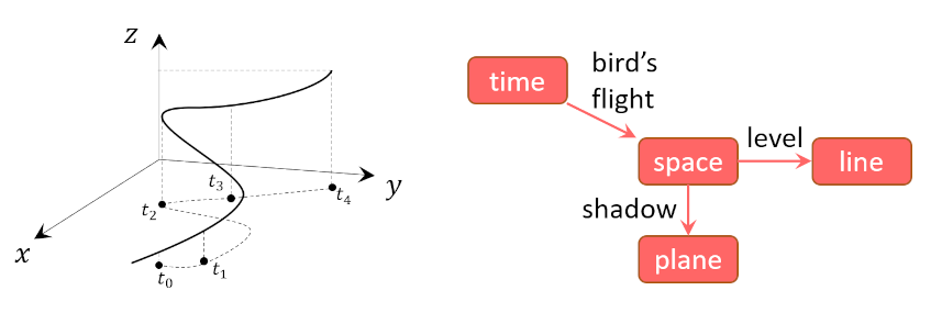
At each instant in time, the bird is at a specific location in space. The physicist’s standard approach is to consider the trajectory as a mapping $f$ from time to space which can symbolically be written as
\[ f:t \rightarrow {\mathbb R}^3 \equiv f:t \rightarrow {\mathbb R} \times {\mathbb R}^2 \; , \]
Where the tensor product in the last relation means that ‘space’ ${\mathbb R}^3$ can be decomposed into ‘line’ ${\mathbb R}$ and ‘plane’ ${\mathbb R}^2$.
I think most physicists stop there with the job accomplished. Being one myself, I pondered for a while what was so important about this point that is deserved a special place in the introduction – the part of the book that a perspective buyer would be most likely to read before purchasing. While I am not completely sold on my interpretation, I believe that the authors were trying to say that the mappings were the basic objects in categories rather than simply the tools to understand the more ‘physical’ objects of time and space.
To further support this interpretation, I’ll point out that the authors list (p 17) the basic ingredients (as they call them) to have a category or ‘mathematical universe’ (again their words). According to this terminology, these ingredients are
Data for the category:
- Objects/sets: $A$, $B$, $C$, $\ldots$
- Maps between sets: $f:A \rightarrow B$ or, synonymously $A \xrightarrow{f} B$. The maps only have one stipulation, that every element in the domain $A$ goes to some element in the range (or codomain) $B$.
- Identity Maps (one per object): $A \xrightarrow{i_A} A$
- Composition of Maps: assigns to each pair of compatible maps (say a map from $f:A \rightarrow B$ followed by another map from $g:B \rightarrow C$) a single map that accomplishes the job at one go (a map directly from $h: A \rightarrow C$) with $h \equiv g \circ f$ read as $g$ follows $f$
Rules for the category
- The identity laws
- If $A \xrightarrow{i_A} A \xrightarrow{g} B$, then $A \xrightarrow{g \circ i_A} B$
- If $A \xrightarrow{f} B \xrightarrow{i_B} B$, then $A \xrightarrow{i_B \circ f} B$
- The associative law
- If $A \xrightarrow{f} B \xrightarrow{g} C \xrightarrow{h} D$, then $A \xrightarrow{h \circ (g \circ f) = (h \circ g) \circ f} D$
They emphasize that the rules, are important, even crucial. I take it that they mean that the key insight is the action between the maps and not the objects the maps relate and that is why I characterize the rules for categories as meta-rules.
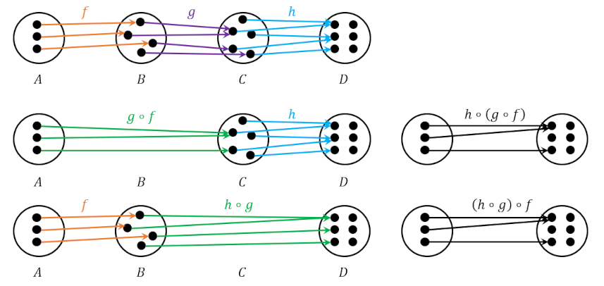
These meta-rules center on the composition of the maps. The identity laws are fairly straightforward with one caveat. The two identity map rules are required since the maps are not required to be bijections, unlike the usual case in physics where the maps are almost always bijections. This extra freedom makes a little more difficult to think about the associativity rule. The following diagram, adapted from the exercises starting on page 18, shows that even in the absence of clear inverse for each map associativity holds; if ones starts with some element in the first set it has to go somewhere in the last set and it doesn’t matter if one thinks of grouping the intermediate steps one way or the other.
The final observation is that the authors make a point that there is a strong analogy between the multiplication of real numbers and the composition of maps. This analogy derives from the combinatorics associated with the way in which one can relate $n$ elements in one set to $m$ elements in another.
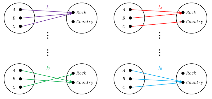
Mathematically, the number of different maps between $A$ and $B$ is given in terms of the number of elements in each (denoted by $N_A$ and $N_B$ respectively) by
\[ {N_B}^{N_A} \; , \]
which for the case in the diagram above is $ 2^3 = 8$ as expected.
The exact insights that this analogy provides remain still a mystery but there is always next month.