
Category Theory 6 – Coding Up Mappings
This month’s article is a bit of a departure from the previous installments on category theory in that it deals with the computational side of things rather than the theoretical side of things. But, as the recent columns have shown, it is typically the case that working with specific examples facilitates a basic understanding of the general.
As a case in point, consider the set of all possible mappings between the sets $A$, $B$, and $C$, an example of which is shown below
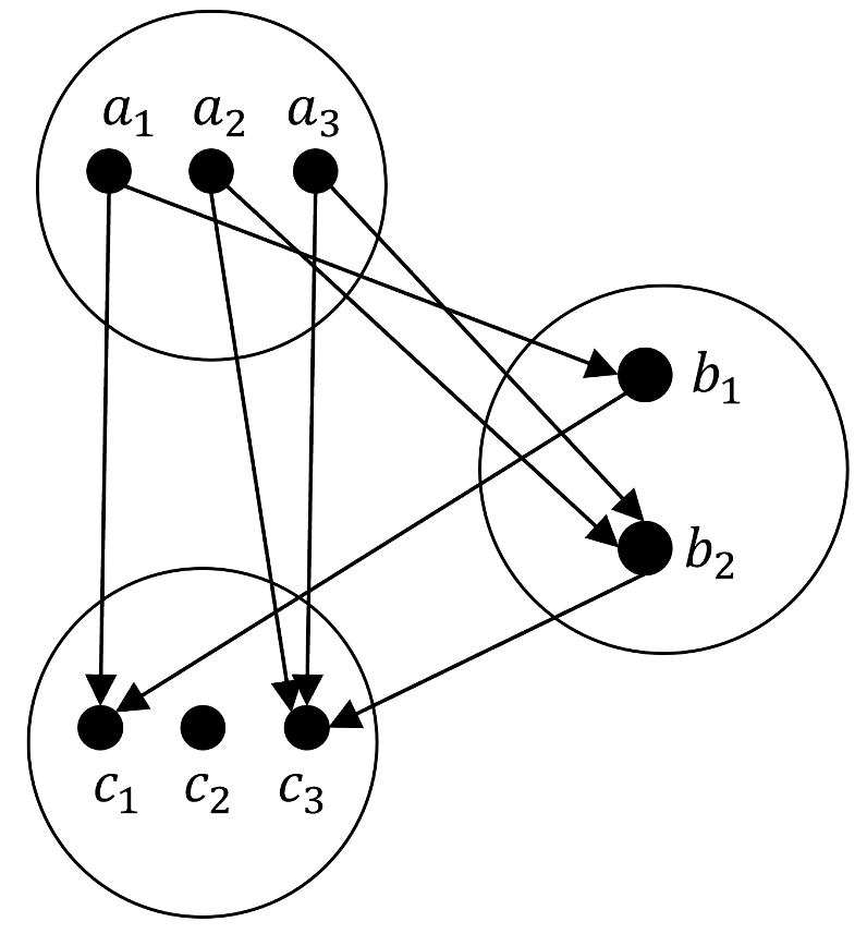
where $A$ has three elements $\left\{ a_1, a_2, a_3\right\}$, $B$ has two elements $\left\{ b_1, b_2 \right\}$, and $C$ has three elements $\left\{ c_1, c_2, c_3\right\}$. Although we’ve focused on automorphisms wherein we identified $A$ and $C$ as the same set, the general case will be what we tackle here.
Even though these sets are small, the combinatorics associated with all possible mappings quickly daunts the use of paper and pencil. There are 8 distinct mappings $f:A \rightarrow B$ and 9 distinct mappings from $g:B \rightarrow C$ leaving 72 mappings in total for the composition. Obviously this situation calls for some basic computing.
Despite the simplicity of the discussion up to date in Lawvere and Schanuel, one thing they didn’t do is actually adopt terminology well-suited to writing computer code. The word ‘set’, of course, is perfect for describing the collection, so that’s okay, but what to call the contents of each set. The typical mathematical terminology would be members or elements but the former has an object-oriented connotation that would tend to obscure things while the latter is simply too generic. In addition, both of those are rather long to type and really don’t speak to what the diagram looks like. For the purposes here, things like $a_3$ or $b_1$ will be called dots since they are represented as such in the diagrams. At this point, their terminology fails and the thing that connects two dots doesn’t even have a name in their bestiary. Since it is drawn as an arrow in the diagrams, that is the name that will be used in the code. The end of the arrow without the point will be called the outgoing side; the end with the point is the incoming side.
Using this terminology, we then say that:
- each set is made up of dots,
- each dot supports one outgoing arrow
- each dot can receive any number of incoming arrows, including zero
- a mapping is a collection of arrows
The python programming language is an excellent choice and everything that follows is done in version 3.x within the Jupyter notebook framework. The sets discussed above are represented as python lists:
Aset = ['a1','a2','a3']
Bset = ['b1','b2']
Cset = ['c1','c2','c3']
The first function
def generate_arrows(set1,set2):
    arrows = []
    for dot1 in set1:
        for dot2 in set2:
            arrows.append(dot1+'->'+dot2)
    return arrows
returns a list of all possible ways to draw arrows from set1 to set2. Applying this function to sets $A$ and $B$ gives:
generate_arrows(Aset,Bset)
['a1->b1', 'a1->b2', 'a2->b1', 'a2->b2', 'a3->b1', 'a3->b2']
This helper function is used by the larger function
def generate_mappings(set1,set2):
    import itertools as it

    arrows      = generate_arrows(set1,set2)
    mapping_gen = it.combinations(arrows,len(set1))
    mappings    = []
    for candidate in mapping_gen:
        count = []
        for i,dot1 in zip(range(len(set1)),set1):
            count.append(0)
            for arrow in candidate:
                if dot1 in arrow:
                    count[i] += 1
        if min(count) != 0:
            mappings.append(candidate)
    return mappings
The function generate_mappings depends on the itertools module in python to determine all the possible combinations to make a mapping. When applied to $A$ and $B$, the output of
A_to_B = generate_mappings(Aset,Bset)

[('a1->b1', 'a2->b1', 'a3->b1'),
 ('a1->b1', 'a2->b1', 'a3->b2'),
 ('a1->b1', 'a2->b2', 'a3->b1'),
 ('a1->b1', 'a2->b2', 'a3->b2'),
 ('a1->b2', 'a2->b1', 'a3->b1'),
 ('a1->b2', 'a2->b1', 'a3->b2'),
 ('a1->b2', 'a2->b2', 'a3->b1'),
 ('a1->b2', 'a2->b2', 'a3->b2')]
is a list 8 elements in length as expected. Each line is one possible mapping between the two sets. Likewise, the total listing of all mappings from $B$ to $C$
[('b1->c1', 'b2->c1'),
 ('b1->c1', 'b2->c2'),
 ('b1->c1', 'b2->c3'),
 ('b1->c2', 'b2->c1'),
 ('b1->c2', 'b2->c2'),
 ('b1->c2', 'b2->c3'),
 ('b1->c3', 'b2->c1'),
 ('b1->c3', 'b2->c2'),
 ('b1->c3', 'b2->c3')]
has 9 possibilities, also as expected.
In order to compose functions, we need a way of combining expressions like ‘a1->b1’ and ‘b1->c3’ to get ‘a1->c3’. This is provided by
def compose_arrows(arrow1,arrow2):
    head1,targ1 = arrow1.split('->')
    head2,targ2 = arrow2.split('->')
    if targ1 == head2:
        return head1+'->'+targ2
    else:
        return False
Note that if the middle term is not the same the function returns a False.
The functionality is rounded out with the
def compose_mappings(mappings1,mappings2):
    mappings = []
    for f in mappings1:
        for g in mappings2:
            compositions = []
            for f_arrow in f:
                for g_arrow in g:
                     compositions.append(compose_arrows(f_arrow,g_arrow))
            while(False in compositions):
                compositions.remove(False)
            mappings.append(tuple(compositions))
    return mappings
which composes two lists of mappings. Plugging in the previous two lists of mappings (mappings = compose_mappings(A_to_B,B_to_C)) gives a list with 72 elements. Of course, given the sizes of $A$ and $C$ there can be, at most, only 27 unique ones. The repetitions are trivially removed by casting the list to a set and then casting it back to a list. Doing this gives the following list of unique mappings:
[('a1->c1', 'a2->c2', 'a3->c1'),
 ('a1->c2', 'a2->c3', 'a3->c2'),
 ('a1->c3', 'a2->c2', 'a3->c3'),
 ('a1->c2', 'a2->c1', 'a3->c2'),
 ('a1->c1', 'a2->c3', 'a3->c1'),
 ('a1->c3', 'a2->c3', 'a3->c1'),
 ('a1->c2', 'a2->c2', 'a3->c3'),
 ('a1->c1', 'a2->c1', 'a3->c1'),
 ('a1->c3', 'a2->c1', 'a3->c1'),
 ('a1->c3', 'a2->c2', 'a3->c2'),
 ('a1->c3', 'a2->c1', 'a3->c3'),
 ('a1->c1', 'a2->c1', 'a3->c3'),
 ('a1->c3', 'a2->c3', 'a3->c3'),
 ('a1->c1', 'a2->c3', 'a3->c3'),
 ('a1->c2', 'a2->c1', 'a3->c1'),
 ('a1->c1', 'a2->c1', 'a3->c2'),
 ('a1->c2', 'a2->c2', 'a3->c1'),
 ('a1->c3', 'a2->c3', 'a3->c2'),
 ('a1->c2', 'a2->c3', 'a3->c3'),
 ('a1->c2', 'a2->c2', 'a3->c2'),
 ('a1->c1', 'a2->c2', 'a3->c2')]
There are 21 in all, 6 less than the 27 possible mappings between $A$ and $C$. The missing ones correspond to the one-to-one mappings between $A$ and $C$ (i.e., $a_1 \rightarrow c_1$, $a_2 \rightarrow c_2$, $a_3 \rightarrow c_3$ and permutations). Of course, these results drive home the point that, since the size of $B$ is smaller than $A$ and $C$, there is simply no way to support a one-to-one mapping.
One can experiment with replacing $B$ with a 4-element set $D$. Doing so gives the expected 27 unique mappings $f: A \rightarrow C$ (at the expense of calculating 5184 possible combinations of going from $A$ to $C$ with a layover at $D$. Obviously nobody should want to do this by hand.
So there you have it: while not theoretically glamorous, functionality like this really allows for an exploration that couldn’t be done by hand.