
Monte Carlo Integration – Part 1
It is a peculiar fact that randomness, when married with a set of deterministic rules, often leads to richness that is absent in a set of deterministic rules by themselves. (Of course, there is no richness in randomness by itself – just noise). An everyday example can be found in the richness of poker that exceeds the mechanistic (albeit complex) rules of chess. This behavior carries over into the realm of numerical analysis where Monte Carlo integration presents a versatile method of computing the value of definite integrals. Given the fact that most integrands don’t have an anti-derivative, this technique can be very powerful indeed.
To understand how it works, consider a function $g(x)$, which is required to be computable over the range $(a,b)$, but nothing else. We will now decompose this function in a non-obvious way
\[ g(x) = \frac{f(x)}{p(x)} \; , \]
where $p(x)$ is a normalized function on the same interval
\[ \int_a^b dx p(x) = 1 \; . \]
If we draw $N$ realizations from $p(x)$
\[ x_1, x_2, \ldots, x_N \; \]
and we evaluate $g(x)$ at each value
\[ g_1, g_2, \ldots, g_N \; , \]
where $g_i \equiv g(x_i)$.
On one hand, the expected value is
\[ E[g(x)] = \frac{1}{N} \sum_i g_i \equiv {\bar g} .\]
This is the empirical value of the sampling of $g(x)$ according to $p(x)$.
The theoretical value is
\[ E[g(x)] = \int_a^b dx p(x) g(x) = \int_a^b dx p(x) \frac{f(x)}{p(x)} = \int_a^b dx f(x) \; . \]
So, we can evaluate the integral
\[ I = \int_a^b dx f(x) \; \]
by sampling and averaging $g(x)$ with a sampling realization of $p(x)$.
The simplest probability distribution to consider is uniform on the range
\[ p(x) = \frac{1}{b -a} \; \]
and with $g(x) = (b-a) f(x)$ we can evaluate
\[ I = \int_a^b dx f(x) = \frac{1}{N} \sum_i g_i = \frac{b-a}{N} \sum_i f_i \; , \]
where $f_i \equiv f(x_i) $.
Before pressing on with the theory, let’s take a look at some specific examples.
For the first example, let’s look at the polynomial
\[ f_p(x) = 3.4 x^3 – 5.9 x^2 + 0.3 x – 15.2 \; \]
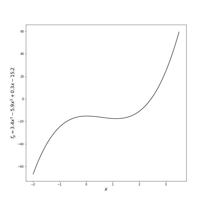
This function has the antiderivative
\[ F_p(x) = \frac{3.4}{4} x^4 – \frac{5.9}{3} x^3 + \frac{0.3}{2} x^2 – 15.2 x \; . \]
The integral of $f_p$ from $x_{min} = -2$ to $x_{max} = 3.5$ has the exact value
\[ \int_{x_{min}}^{x_{max}} dx f_p = F_p(x_{max}) – F_p(x_{min}) = -68.46354166666669 \; . \]
A simple script in python using numpy, scipy, and a Jupyter notebook was implemented to explore numerical techniques to perform the integral. The scipy.integrate.quad function, which uses traditional quadrature based on the Fortran QUADPACK routines, returned the value of -68.46354166666667, which is exactly (to within machine precision) the analytic result. The Monte Carlo integration, which is implemented with the following lines
N = 100_000
rand_x = x_min + (x_max - x_min)*np.random.random(size=N)
rand_y = f(rand_x)
I_poly_est  = (x_max - x_min)*np.average(rand_y)
returned a value of -68.57203483190794 using 100,000 samples (generally called a trial – a terminology that will be used hereafter) with a relative error of 0.00158. This is not bad agreement but clearly orders of magnitude worse than the deterministic algorithm. We’ll return to this point later.
One more example is worth discussing. This time the function is a nasty, nested function given by
\[ f_n = 4 \sin \left( 2 \pi e^{\cos x^2} \right) \; , \]
which looks like

over the range $[-2,3.5]$. Even though this function doesn’t have an anti-derivative, its integral clearly exists since the function is continuous with no divergences. The deterministic algorithm found in scipy.integrate.quad generates the value of -2.824748541066965, which we will take as truth. The same Monte Carlo scheme as above yields a value -2.8020549889975164 or relative error 0.008034.
So, we can see that the method is versatile and reasonably accurate. However, there are two questions that one might immediately pose: 1) why use it if there are more accurate methods available and 2) can the estimates be made more accurate? The remainder of this post will deal with answering question 1 while the subsequent post will answer the second question.
To answer question 1, we will cite, without proof, the answer to question 2 that states the error $\epsilon$ in the estimate of the integral goes to zero as the number of samples according to
\[ \epsilon \sim \frac{1}{\sqrt{N}} \; \]
independent of the number of dimensions.
To determine the error for a conventional quadrature method (e.g. trapezoidal or Simpson’s), we follow the argument from Steve Koonin’s Computational Physics p 201. Assume that we will evaluate the integrand $N$ times (corresponding to the $N$ times it will be evaluated with the Monte Carlo scheme). The $d$-dimensional region over for the integral consists of a volume ${V} ~ {h}^d$. Distributing the $N$ points over the volume means that the grid spacing $h ~ N^{-1/d}$.
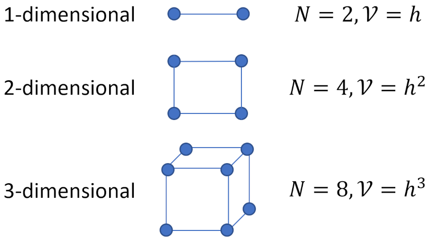
Koonin states that an analysis similar to those used for the usual one-dimensional formulae gives the error as going $O\left(h^{d+2}\right)$. The total error of the quadrature thus goes as
\[ N O\left(h^{d+2}\right) = O\left(N^{-2/d}\right) \; .\]
When $d \geq 4$, the error in estimating the integral via Monte Carlo becomes smaller than that for standard quadrature techniques for a given computing time invested. This reason alone justifies why the Monte Carlo technique is so highly favored. In particular, Monte Carlo proves invaluable in propagating variations through dynamical systems whose dimensionality precludes using a gridded method like traditional quadrature.
The next post will derive why the Monte Carlo error goes as $1/\sqrt(N)$.