
Monte Carlo Integration – Part 2
The last post introduced the basic concept of Monte Carlo integration, which built on the idea of sampling the integrand in a structured (although random) way such that the average of the samples, appropriately weighted, estimates the value of a definite integral. This method, while not as accurate for lower-dimensional integrals (for a given invested amount of computer time) as the traditional quadrature techniques (e.g., Simpson’s rule), really shines for problems in 4 or more dimensions. (Note: The method also works well for multiple integrals in 2 and 3 dimensions when the boundary is particularly complex.) This observation is based on the fact that the error in the Monte Carlo estimation goes as $1/\sqrt{N}$, $N$ being the number of samples, independent of the number of dimensions.
This post explores the error analysis of the Monte Carlo method and demonstrates the origin of the $1/\sqrt{N}$ dependence.
The first step is simply to look at how the error in the estimation of the integral varies as a function of the number of samples (hereafter called the number of Monte Carlo trials). The example chosen is the polynomial
\[ f_p(x) = 3.4 x^3 -5.9 x^2 + 0.3 x -15.2 \; \]
used in the previous post. The limits of integration are $x_{min} = -2$ and $x_{max} = 3.5$ and the exact value of this integral is $I_{p} = -68.46354166666669$. The following table shows the error between the exact value and the value estimated using the Monte Carlo sampling method for the number of trials ranging from 100 to 100,000,000 trials. All the data were obtained using a Jupyter notebook running python and the numpy/scipy ecosystem.
| Num Trials | $I_p$ | Error ($\epsilon_p$) |
| 100 | -96.869254 | 28.405712 |
| 1,000 | -67.729511 | 0.734030 |
| 5,000 | -69.960783 | 1.497241 |
| 10,000 | -66.881870 | 1.581672 |
| 50,000 | -67.721144 | 0.742398 |
| 100,000 | -68.327480 | 0.136062 |
| 500,000 | -68.747538 | 0.283996 |
| 1,000,000 | -68.494555 | 0.031013 |
| 10,000,000 | -68.548658 | 0.085116 |
| 100,000,000 | -68.468060 | 0.004519 |
Even though the error generally trends downward as $N$ increases, there are fluctuations associated with the random nature of the sampling process. The figure below shows a log-log scatter plot of these data along with a best fit line to the points.
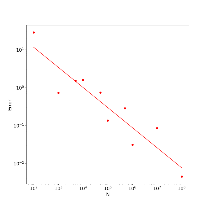
The value of the slope returned by the linear regression was -0.529, very close to the expected value of $-1/2$; the $r^2$ value of the fit was 0.85 indicating that the linear fit very well explained the trend in the points, although it is important to realize that subsequent runs of this numerical experiment will produce different results.
While this result is compelling it lacks in two ways. First, due to the random nature of the sampling, the trend will never be nailed down to be exactly an inverse square root. Second, we had an exact value to compare to and so could quantitatively gauge the error. In practice, we want to use the method to estimate integrals whose exact value is unknown and so we need an intrinsic way of estimating the error.
To address these concerns, we expand on the discussion in Chapter 10 of An Introduction to Computer Simulation Methods, Applications to Physical Systems, Part 2 by Gould and Tobochnik.
In their discussion, the authors considered estimating
\[ I_{circ} = \int_0^1 dx \, 4 \sqrt{1-x^2} = \pi \; \]
multiple times using a fixed number of trials for each estimation. Comparing the spread in the values of each estimation then gives a measure of the accuracy in the estimation. To be concrete, consider the 10 estimations performed using 100,000 trials each. The following table summarizes these cases with the first column being the average, the second the error against the exact value of $\pi$, (a situation, which, in general, we will not have). The third channel is the standard deviation as measure of the spread of the sample used in the estimation. We’ve introduced with hope of it filling the role of an intrinsic estimate of the error.
| $I_{circ}$ | Error ($\epsilon_p$) | Standard Deviation |
| 3.143074 | 0.001481 | 0.892373 |
| 3.146796 | 0.005203 | 0.888127 |
| 3.142626 | 0.001034 | 0.895669 |
| 3.139204 | 0.002389 | 0.893454 |
| 3.145947 | 0.004355 | 0.891186 |
| 3.142209 | 0.000616 | 0.892600 |
| 3.137025 | 0.004568 | 0.896624 |
| 3.136014 | 0.005578 | 0.895747 |
| 3.140397 | 0.001196 | 0.892305 |
| 3.140693 | 0.000900 | 0.892604 |
We can perform some statistical reduction of these data that will serve to direct us further. First of all, the mean estimate (mean of the means) is $\langle I_{circ} \rangle = 3.1413985717765454$ with a standard deviation (sigma of the means) of $\sigma_{\langle I_{circ} \rangle} = 0.003304946237283195$. The average of the standard deviation (mean of the sigmas) is $<\sigma>= 0.8930688485193065$. Finally, the average error $<\epsilon> = 0.0027319130714524853$. Clearly, $\sigma_{\langle I_{circ}\rangle} \approx <\epsilon>$ but both are two orders of magnitude smaller than $<\sigma>$. A closer look reveals that the ratio $<\sigma>/\sigma_{\langle I_{circ}\rangle}$ is approximately $300 \approx 1/\sqrt{100,000}$. This isn’t a coincidence. Rather it reflects the central limit theorem.
The central limit theorem basically says that if we pull $K$ independent samples, each of size $N$, from an underlying population, then regardless of the structure of the population distribution (with some minor restrictions) the distribution of the $K$ averages computed will be Gaussian.
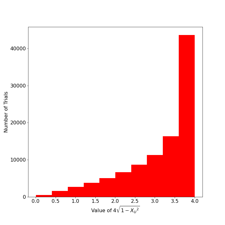
This point is more easily understood with specific examples. Below is a plot of the distribution of values of $4 \sqrt{1 -x^2}$ for a single Monte Carlo estimation with $N=100,000$ trials. The histogram shows a distribution that strongly looks like an exponential distribution.
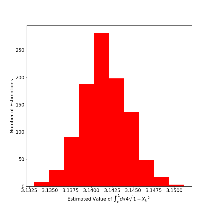
However, when this estimation is repeated so that $K=1,000$ and the distribution of those thousand means are presented in a histogram, the distribution looks strongly like a normal (aka, Gaussian) distribution.
The power behind this observation is that we can then estimate the error in original estimation in terms of the standard deviation of the sample itself. In other words,
\[ \sigma_{\langle I_{circ} \rangle} = \frac{<\sigma>}{\sqrt{N}} \; .\]
The proof of the generalize relation (Appendix 10B of Gould & Tobochnik) goes as follows.
Start with the $K$ independent samples each of size $N$ and form the $K$ independent means as
\[ M_k = \frac{1}{N} \sum_{n=1}^{N} x^{(k)}_n \; ,\]
where $x^{(k)}_n$ is the value of the $n^{th}$ trial of the $k^{th}$ sample.
The mean of the means (i.e. the mean over all $K \cdot N$ trials) is then given by
\[ {\bar M} = \frac{1}{K} \sum_{k=1}^{K} M_k = \frac{1}{K} \sum_{k=1}^{K} \frac{1}{N} \sum_{n=1}^{N} x^{(k)}_n \; .\]
Next define two measures of the difference between the individual measures and the mean of the means: 1) the $k^{th}$ residual, which measures the deviation of an $M_k$ from ${\bar M}$ and is given by
\[ e_k = M_k-{\bar M} \; \]
and 2) the deviation, which is the difference between a single trial and ${\bar M}$, is given by
\[ d_{k,n} = x^{(k)}_n – {\bar M} \; . \]
The residuals and deviations are related to each other as
\[ e_k = \frac{1}{N}\sum_{n=1}^{N} x^{(k)}_n – {\bar M} = \frac{1}{N} \sum_{n=1}^{N} \left( x^{(k)}_n – {\bar M} \right) = \frac{1}{N} \sum_{n=1}^{N} d_{k,n} \; .\]
Averaging the squares of the residuals gives the standard deviation of the ensemble of means
\[ {\sigma_M}^2 = \frac{1}{K} \sum_{k=1}^{K} {e_k}^2 \;. \]
Substituting in the relation between the residuals and the deviations gives
\[ {\sigma_M}^2 = \frac{1}{K} \sum_{k=1}^{K} \left( \frac{1}{N} \sum_{n=1}^{N} d_{k,n} \right) ^2 \; .\]
Expanding the square (making sure to have independent dummy variables for each of the inner sums) yields
\[ {\sigma_M}^2 = \frac{1}{K} \sum_{k=1}^{K} \left( \frac{1}{N} \sum_{m=1}^{N} d_{k,m} \right) \left( \frac{1}{N} \sum_{n=1}^{N} d_{k,n} \right) \; .\]
Since the individual deviations are independent of each other, there should be as many positive as negative terms, and averaging over the terms where $m \neq n$ should result in zero. The only surviving terms are when $m = n$ giving
\[ {\sigma_M}^2 = \frac{1}{K} \frac{1}{N^2} \sum_{k=1}^{K} \sum_{n=1}^{N} d_{k,n}^2 = \frac{1}{N} \left[ \frac{1}{KN} \sum_{k=1}^{K} \sum_{n=1}^N (x^{(k)}_n –{\bar M} )^2 \right] \; . \]
The quantity in the braces is just the standard deviation $\sigma^2$ of the individual trials (regardless to which sample they belong) and so we get the general result
\[ {\sigma_M} = \frac{\sigma}{\sqrt{N}} \; . \]
Next post will examine the implications of this result and will discuss importance sampling as a mechanism to drive the estimated error to a minimum.