
Monte Carlo Integration – Part 3
The last post explored the error analysis for Monte Carlo integration in detail. Numerical experiments indicated that the error in the algorithm goes as $1/\sqrt{N}$, where $N$ are the number of Monte Carlo trials used to make the estimate. Further analysis of the sampling statistics led to a fundamental formula describing the estimated error of the estimated value $\langle I \rangle$ of the integral as
\[ \sigma_{\langle I \rangle } = \frac{\sigma}{\sqrt{N}} \; , \]
where $\sigma$ is the standard deviation of the random process used to evaluate the integral. In other words, we could report the estimated value of some integral as
\[ I = \int_a^{b} \, dx f(x) \approx \frac{1}{N} \sum_{i} \frac{f_i(x)}{p_i(x)} \pm \frac{\sigma}{\sqrt{N}} \; , \]
where $p(x)$ is some known probability distribution. We report this estimate with the understanding that the last term is an estimated $1\sigma$ error of the sampling mean, which is expected to ‘look’ Gaussian as a consequence of the central limit theorem.
While it is attractive to think that an appropriate strategy to improve the estimate of $I$ is to crank up the number of Monte Carlo trials so that the error is as small as desired doing so completely ignores the other ‘knob’ that can be turned in the error equation, namely the value of $\sigma$.
At first, it isn’t obvious how to turn this knob and why we should even consider figuring out how. Motivation comes when we reflect on the fact that in the most important and interesting cases the integrand $f(x)$ may be very or extremely computationally expensive to evaluate. In those cases, we might look for a way to make every Monte Carlo trial count as maximally as it can. Doing so may cut down on run times to get a desired accuracy from days to.
Given that motivation, the next question is how. An illustrative example helps. Consider the integral of a constant integrand, say $f(x)=2$ over the range $0$ to $1$ sampled with a uniform probability distribution. The estimate of the integral becomes
\[ I = \int_0^{1} \, dx 2 \approx \frac{1}{N} \sum_{i} 2 = \frac{2N}{N} = 2 \; , \]
regardless of the number of trials. In addition since each trial returns the same value, the sample standard deviation is $\sigma = 0$. The estimate is exact and independent of the number of trials.
Our strategy for the general $f(x)$ is quite clear; we want to pick the probability measure such that the ratio $f(x)/p(x) = \textrm{constant}$. This strategy is termed importance sampling because the samples are preferentially placed in regions where $f(x)$ is bigger. This isn’t always possible but let’s examine another case where we can actually do this.
Let’s estimate the integral
\[ I = \int_{0}^{1} \, dx \left(1 – \frac{x}{2} \right) = \frac{3}{4} \; .\]
The integrand is linear across the range taking on the values of $1$ when $x=0$ and $1/2$ for $x=1$. We want our probability distribution also be linear over this range but to be normalized. A reasonable choice is to simply normalize the integrand directly, giving
\[ p(x) = \frac{4}{3}\left( 1 – \frac{x}{2} \right) \; .\]
The ratio $f(x)/p(x) = \frac{3}{4}$ and our expectation is that the Monte Carlo integration should give the exact result.
The only detail missing is how to produce a set of numbers taken from that probability distribution. To answer this question let’s follow the discussion in Chapter 8 of Koonin’s Computational Physics and rewrite the original integral in a suggestive way
\[ \int_0^{1} \, dx f(x) = \int_0^{1} \, dx \, p(x) \frac{f(x)}{p(x)} \; . \]
Now, define the cumulative distribution as
\[ y(x) = \int_0^x \, dx’ p(x’) \; \]
and make a change of variables from $x$ to $y$. Using Leibniz’s rule,
\[ \frac{dy}{dx} = p(x) \; , \]
which gives $dx = dy/p(x)$. Turning to the limits of the integral, we find $y(x=0) = 0$ and $y(x=1) = 1$ and the new form of the integral is
\[ \int_0^{1} \, dy \frac{f(y)}{p(y)} \; .\]
We can now tackle this integral by sampling $y$ uniformly over the interval $[0,1]$ as if the integral were originally written this way.
Since $y$ is uniformly distributed, if an anti-derivative exist for $p(x)$ and we can invert the result to express $x=x(y)$ we will automatically get the desired distribution for random realizations of $p(x)$. For the case at hand, $p(x) = \frac{4}{3}\left(1 – \frac{x}{2}\right)$. The expression for $y$ is then
\[ y = \frac{4}{3} \left(x – \frac{x^2}{4} \right) \; .\]
This quadratic equation can be solved for $x$ to give
\[ x = 2- (4- 3y)^{1/2} \; .\]
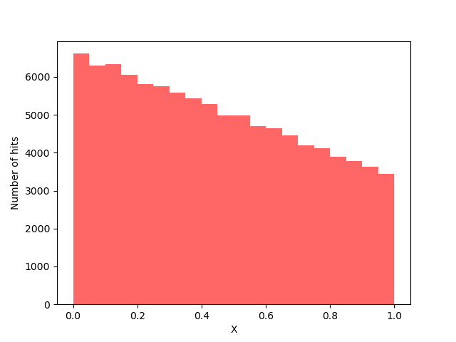
The following figure shows the distribution of $x$ as a random variable given a 100,000 uniformly distributed random numbers representing $y$.
All of this machinery is easily implemented in python to provide a side-by-side comparison between directly sampling the original integral using both a uniform distribution and the importance sampling using the linear distribution.
import matplotlib as mpl
import numpy      as np
import pandas     as pd
import scipy      as sp
import matplotlib.pyplot as plt
Ns   = [10,20,50,100,200,500,1_000,2_000,5_000,10_000,100_000]
xmin = 0
xmax = 1
df   = pd.DataFrame()
def f(x): return (1.0 - x/2.0)
def w(x): return (4.0-2.0*x)/3.0
def x(x): return 2.0 - np.sqrt(4.0 - 3.0*x)
for N in Ns:
    y   = np.random.random((N,))
    Fu  = f(y)
    X   = x(y)
    Wx  = w(X)
    Fx  = f(X)
    row = {'N':N,'I_U':np.mean(Fu),'sig_I_U':np.std(Fu)/np.sqrt(N),\
          'I_K':np.mean(Fx/Wx),'sig_I_K':np.std(Fx/Wx)/np.sqrt(N)}
    df = df.append(row,ignore_index=True)
print(df)
The following table shows the results from this experiment (i.e. the contents of the pandas dataframe).
| $N$ | $I_U$ | $\sigma_{I_U}$ | $I_L$ | $\sigma_{I_L}$ |
| 10 | 0.811536 | 0.052912 | 0.75 | 0.0 |
| 20 | 0.787659 | 0.033866 | 0.75 | 0.0 |
| 50 | 0.768951 | 0.020441 | 0.75 | 0.0 |
| 100 | 0.755852 | 0.014472 | 0.75 | 0.0 |
| 200 | 0.752533 | 0.010497 | 0.75 | 0.0 |
| 500 | 0.749750 | 0.006580 | 0.75 | 0.0 |
| 1000 | 0.749777 | 0.004602 | 0.75 | 0.0 |
| 2000 | 0.745935 | 0.003184 | 0.75 | 0.0 |
| 5000 | 0.748036 | 0.002035 | 0.75 | 0.0 |
| 10000 | 0.751155 | 0.001438 | 0.75 | 0.0 |
| 100000 | 0.749597 | 0.000457 | 0.75 | 0.0 |
It is clear that the estimate of the integral $I_U$ slowly converges to the exact value of $3/4$ but that by matching the importance sampling weight $p(x)$ such that $f(x)/p(x)$ is a constant, we get an exact value $I_L$ of the integral with no uncertainty.
Of course, this illustrative example is not meant to be considered a triumph since we had to know the exact value integral to determine $p(x)$ in the first place. But it does point to applications where we either don’t or can’t evaluate the integral.
In the next post, we’ll explore some of these applications by looking at more complex integrals and discuss some of the specialized algorithms designed to exploit importance sampling.