
Monte Carlo Integration – Part 4
In the last installment, we touched on the first rudiments of importance sampling as a way of improving the Monte Carlo estimation of integrals. The key relationship is that a Monte Carlo estimate of an integral $I$ is given
\[ I = \int_a^b \, dx \, f(x) \approx \frac{1}{N} \sum_i \frac{f(x)}{p(x)} \pm \frac{\sigma}{\sqrt{N}} \; , \]
where $p(x)$ is a known probability distribution and $N$ are the number of Monte Carlo trials (i.e. random samples).
The error in the estimate depends on two terms: the number of Monte Carlo trials $N$ and the sample standard deviation $\sigma$ pulled at random from $p(x)$. Although the error in the estimation can be made as small as possible by increasing the number of trials, the convergence is rather slow. The importance sampling strategy is to make each Monte Carlo trial count as much as possible by adapting $p(x)$ to the form of $f(x)$ such that the ratio of the two terms is a close as possible to being a constant.
The examples of how to implement this strategy from the last post were highly contrived to illustrate the method but are not representative of what is actually encountered in practice since the majority of integrands are complicated and often no able to even be represented in closed form.
In this post, we are going to extend this method a bit by considering examples where the ratio of $f(x)/p(x)$ is not a constant.
Our first example will be to estimate the integral
\[ I = \int_{0}^{10} \, dx \, e^{-x^2} \; . \]
Up to an overall scaling this integral is proportional to the error function defined as
\[ erf(z) = \frac{2}{\sqrt{\pi}} \int_0^z \, dx e^{-x^2} \; . \]
While the error function is special function that can’t be expressed as a finite number of elementary terms, it has been studied and cataloged and, like the trigonometric functions, can be thought of as being a known function with optimized ways of getting a numerical approximation. Our original integral is then
\[ I = \frac{\sqrt{\pi}}{2} erf(10) \approx 0.886226925452758 \; , \]
which we take as the exact, “truth” value.
To start we are going to estimate this integral using two different probability distributions: the uniform distribution, to provide the naïve Monte Carlo baseline for comparison, and the exponential distribution $p(x) \propto \exp(-x)$. While the exponential distribution doesn’t exactly match the integrand (i.e. $exp(-x^2)/exp(-x) \neq \textrm{constant}$), it falls off similarly
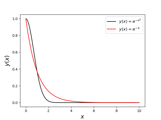
and will provide a useful experiment to set expectations of what the performance will be when $p(x)$ only approximately conforms to $f(x)$. Using the exponential distribution will also provide another change to use the variable substitution method for generating probability distributions.
To generate an exponential distribution, we assume $y$ random variable related to the random variable $x$ through an integral where the exponential distribution is the integrand
\[ y = \int_{0}{x} \, dt e^{-t} \; .\]
Since $y$ is the cumulative distribution function it sits on the range $[0,1]$ and when it is uniformly distributed $x$ will be exponentially distributed. The only remaining step is to express $x$ in terms of $y$. For the exponential distribution, this is easily done as the integral is elementary. Carrying out that integration gives
\[ y = \left. – e^{-t} \right|_{0}^{x} = 1 – e^{-x} \; .\]
Solving for $x$ yields
\[ x = -\ln (1-y) \; .\]
This relation is very simple to implement in python and a $N=10,000$ set of uniform random numbers for $y$ results the following histogram for the distribution for $x$,
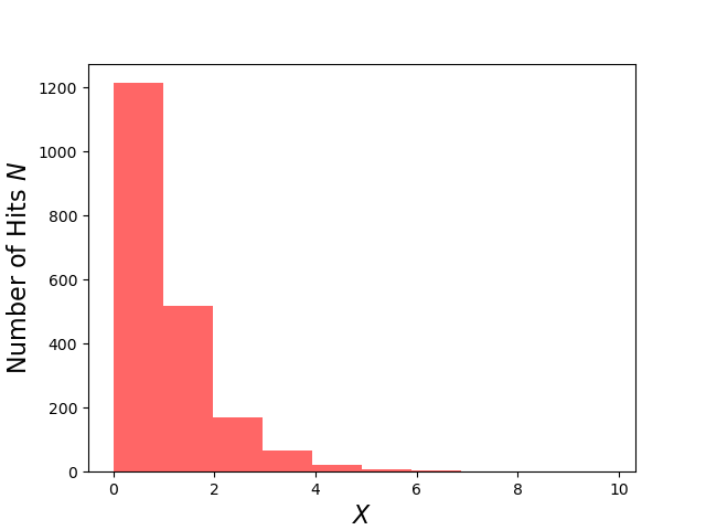
which has a mean of $s_x = 1.00913$ and a $\sigma_x = 0.98770$ compared to the exact result for both being $1$.
Of course, most programming languages have optimized forms of many distributions and python is no different so we could have used the built-in method for the exponential distribution. Nonetheless, following the above approach is important. Understanding this class of method in detail reveals when it can and cannot work and illustrates some of the difficulties encountered in generating pseudorandom numbers from arbitrary distributions. It helps to explain why some distributions are ‘built-in’ (e.g. the exponential distribution) when others, say a distribution proportion to a fifth-order or higher order polynomial over a finite range, are not. It also provides a starting point for considering how to create distributions that are not analytically tractable.
With the exponentially-distributed pseudorandom numbers in hand, we can then estimate the integral with the importance sampling method and compare it to using naïve uniformly-distributed Monte Carlo. The code I used to perform this comparison is:
Ns   = [i for i in range(10,2010,10)]
xmin = 0
xmax = 10
df   = pd.DataFrame()

#exact answeer for this integral in terms of the error function
exact = np.sqrt(np.pi)/2.0*special.erf(10)

def f(x): return np.exp(-x*x)
def pu(span): return 1/(span[1]-span[0])
def pe(x): return np.exp(-x)
def xk(x): return -np.log(1-x)

for N in Ns:
    U = np.random.random((N,))
    FU = f(xmin + xmax*U)
    PU = pu((xmin,xmax))
    XK = xk(U)
    PE = pe(XK)
    FX = f(XK)

    mean_U = np.mean(FU/PU)
    sig_U  = np.std(FU/PU)/np.sqrt(N)
    err_U  = mean_U - exact
    mean_K = np.mean(FX/PE)
    sig_K  = np.std(FX/PE)/np.sqrt(N)
    err_K  = mean_K - exact

    row = {'N':N,\
           'I_U':mean_U,\
           'sig_I_U':sig_U,\
           'error_U':err_U,\
           'I_K':mean_K,\
           'sig_I_K':sig_K,\
           'error_K':err_K}
    df  = df.append(row,ignore_index=True)
Each record of the dataframe df contains the number of Monte Carlo trials $N$ as well as the estimated value of the integral, the uncertainty for both the uniform and importance-sampled estimators, and their corresponding actual error, respectively. The following plot shows the error in the estimated value of the integral
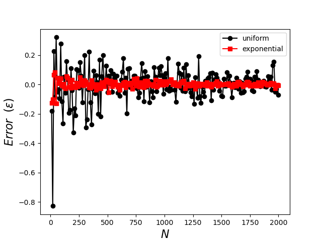
clearly demonstrating the superior performance of the importance sampling with the exponential distribution, which converges rapidly for small $N$ and which exhibits less tendency to fluctuate as well. The plot of standard deviation shows similar performance
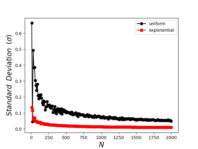
with the standard deviation in the exponential sampling falling much faster as a function of $N$ and achieving a smaller and smoother overall value. The standard deviation, which is the only measure one has when the exact value of the integral is unknown, is often called the formal error as it is taken as a proxy for the exact error.
Next month we’ll discuss some of use cases where the estimation of high-dimensional integrals necessitates importance sampling and the high-powered algorithms that can be plugged-in (sometimes with some effort).