
Sunny Day Markov Chain
In the last post, we demonstrated that not all conditional probabilities are conceptually equal even if they are linguistically equal. The specific case discussed at the end – the sunny day case – doesn’t fit the usual mold. To better understand why it doesn’t fit let’s looks back at the textbook case.
Ordinarily, we calculate a conditional probability by fixing one of the variables from a joint probability distribution and renormalizing so that ‘the probability of $B$ given $A$’, denoted by $P(B|A)$ obeys all the axioms of probability theory. For simplicity, the joint probability distribution in the previous analysis was presented as a table (e.g. color and life of a bulb or snack preference based on sex) but any mathematically multi-variate function capable of being normalized serves.
But the sunny day case is different. In that case, we define transition probabilities that express what the chance that the weather tomorrow will be like given the weather today, where there were only two possible outcomes: ‘Sunny’ (denoted as $S$) and ‘Rainy’ (denoted as $R$). The conditional probabilities were:
\[ P(S|S) = 0.9 \; \]
and
\[ P(R|S) = 0.1 \; , \]
for the weather tomorrow based on today’s weather being sunny. Likewise,
\[ P(S|R) = 0.5 = P(R|R) \; ,\]
given that today is rainy.
It isn’t all clear how many actual variables we have in the joint probability distribution. Is it 2, one for today and one for tomorrow? Clearly that’s wrong since in any given span of days, say the month of September, taken in isolation, there are 28 days that serve as both a today and a tomorrow and 1 day each that is either a tomorrow or a today but not both. As we’ll see below, in a real sense there are an infinite number of variables in the joint distribution since there are limitless todays and tomorrows (ignoring the obvious conflict with modern cosmology).
The question left hanging was just how could we determine the probability that, given an $N$-day long span of time, the weather on any given day was sunny.
This type of problem is called a Markov chain problem defined as the type of problem where the transition probabilities only depend on the current state and not something further back. This type of system is said to have no memory.
There are two equally general methods for computing the long term probability of any given day being sunny or rainy but they differ in convenience and scope. The first is the analytic method.
In the analytic method, we express the state of the system as a vector ${\bar S}$ with two components stating the probability of getting a sunny or rainy day. The transition rules express themselves nicely in matrix form according to
\[ {\bar S}_{tomorrow} = M {\bar S}_{today} \; ,\]
which has the explicit form
\[ \left[ \begin{array}{c} S \\ R \end{array} \right]_{tomorrow} = \left[ \begin{array}{cc} 0.9 & 0.5 \\ 0.1 & 0.5 \end{array} \right] \left[ \begin{array}{c} S \\ R \end{array} \right]_{today} \; . \]
The explicit form of $M$ can be checked against an initial, known state of either ${\bar S}^{(0)} = [1,0]^{T}$ for sunny or ${\bar S}^{(0)} = [0,1]^{T}$ for rainy.
The matrix $M$ links the weather state today to that of tomorrow and we can think of it as an adjacency matrix for the following graph
with the interpretation that the edge weightings are the conditional transition probabilities.
Now lets place an index on any given day just to keep track. The state of the nth day is related to the initial state by
\[ {\bar S}^{(n)} = M {\bar S}^{(n-1)} = M^n {\bar S}^{0} \; .\]
Since we would like to know the probability of picking a sunny day from a collection of days, we are looking for a steady state solution, one which is immune to random fluctuations associated with a string of good or bad luck. This special state ${\bar S}^{*}$ must correspond to $n \rightarrow \infty$ and so it must remain unchanged by successive applications of $M$ (otherwise it doesn’t represent a steady state). Mathematically, this condition can be expressed as
\[ {\bar S}^{*} = M {\bar S}^{*} \; , \]
or, in words, ${\bar S}^{*}$ is an eigenvector of $M$. Computing the eigenvectors of $M$ is easy with numpy and the results are
\[ {\bar S}^{*}_{\lambda_1} = [0.98058068, 0.19611614]^{T} \; \]
and
\[ {\bar S}^{*}_{\lambda_2} = [-0.70710678, 0.70710678]^{T} \; \]
for $\lambda_1 = 1$ and $\lambda_2 = 0.4$. We reject the vector corresponding to $\lambda_2$ because it has negative entries which can’t be interpreted as probabilities. All that is left is to scale ${\bar S}^{*}_{\lambda_1}$ so that the sum of the entries is 1. Doing so gives,
\[ {\bar S}^{*} = [0.8333{\bar 3},0.16666{\bar 6}]^{T} \; ,\]
where the subscript has been dropped as it serves no purpose.
While mathematically correct, one might feel queasy about $\lim_{n\rightarrow \infty} M^n$ converging to something meaningful. But a few numerical results will help support this argument. Consider the following 3 powers of $M$
\[ M^2 = \left[ \begin{array}{cc} 0.86 & 0.70 \\ 0.14 & 0.3 \end{array} \right] \; ,\]
\[ M^{10} = \left[ \begin{array}{cc} 0.83335081 & 0.83324595 \\ 0.16664919 & 0.16675405 \end{array} \right] \; ,\]
and
\[ M^{20} = \left[ \begin{array}{cc} 0.83333334 & 0.83333332 \\ 0.16666666 & 0.16666668 \end{array} \right] \; .\]
Clearly, repeated powers are causing the matrix to converge and the elements that obtain in the limit are the very probabilities calculated above and, by the time $n=20$ we have essentially reached steady state.
The second method is numerical simulation where we ‘propagate’ an initial state forward in time according to the following rules:
- draw a uniform random number in the range $P \in [0,1]$ (standard range)
- if the current state is $S$ then
- set the new state to $S$ if $P \leq 0.9$
- else set the new state to $R$
- if the current state is $R$ then
- set the new state to $S$ is $P \leq 0.5$
- else set the new state to $R$
- Record the new state and repeat
An alternative way of writing the same thing reads
- draw a uniform random number in the range $P \in [0,1]$ (standard range)
- if the current state is $S$ then
- set the new state to $R$ if $P \leq 0.1$
- else set the new state to $S$
- if the current state is $R$ then
- set the new state to $R$ is $P \leq 0.5$
- else set the new state to $R$
- Record the new state and repeat
Of course, hybridizations of these rule sets where block 2 in the first set if matched with block 3 in the second and vice versa also give the same results. It is a matter of taste.
In any event, these rules are easy to implement in python and the following plot shows the fraction of $S$’s as a function of the number of times the rule has been implemented
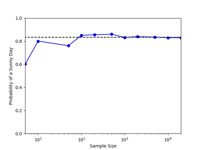
The dotted line shows the value for the probability of a sunny day obtained from the first method and clearly the simulations shows that it converges to that value. This sunny/rainy day simulation is an example of Markov Chain Monte Carlo, which will be the subject of upcoming blogs.