
Metropolis-Hastings I
The last two columns explored the notion for transition probabilities, which are conditional probabilities that express the probability of a new state being realized some system given the current state that the system finds itself in. The candidate case that was examined involved the transition probabilities of between weather conditions (sunny-to-rainy, sunny-to-sunny, etc.). That problem yielded answers via two routes: 1) stationary analysis using matrix methods and 2) Markov Chain Monte Carlo (MCMC).
The analysis of the weather problem left one large question looming. Why anyone would ever use the MCMC algorithm when the matrix method was both computationally less burdensome and also gave exact results compared to the estimated values that naturally arise in an Monte Carlo method.
There are many applications but the most straightforward one is the Metropolis-Hasting algorithm for producing pseudorandom numbers from an arbitrary distribution. In an earlier post, we presented an algorithm for producing pseudorandom numbers within a limited class of distributions using the Inverse Transform Method. While extremely economical the Inverse Transform Method depends on the finding invertible relationship between a uniformly sampled pseudorandom number $y$ and the variable $x$ that we want distributed according to some desired distribution.
The textbook example of the Inverse Transform Method is the exponential distribution. The set of pseudorandom numbers given by
\[ x = -\ln (1-y) \; , \]
where $y$ is uniformly distributed on the interval $[0,1]$, is guaranteed to be distributed exponentially.
If no such relationship can be found, the Inverse Transform Method fails to be useful.
The Metropolis-Hastings method is capable to overcoming this hurdle at the expense of being computationally much more expensive. The algorithm works as follows:
- Setup
- Select the distribution $f(x)$ from which a set random numbers are desired
- Arbitrarily assign a value to a random realization $x_{start}$ of the desired distribution consistent with its range
- Select a simple distribution $g(x|x_{cur})$, centered on the current value of the realization from which to draw candidate changes
- Execution
- Draw a change from $g(x|x_{cur})$
- Create a candidate new realization $x_{cand}$
- Form the ratio $R = f(x_{cand})/f(x_{cur})$
- Make a decision as the keeping or rejecting $x_{cand}$ as the new state to transition to according to the Metropolis-Hastings rule
- If $R \geq 1$ then keep the change and let $x_{cur} = x_{cand}$
- If $R < 1$ then draw a random number $q$ from the unit uniform distribution and make the transition if $q < R$
The bulk of this algorithm is very straightforward and simple. The only confusing part is the Metropolis-Hastings decision rule in the last step and why it requires the various pieces above to work. The next post will be dedicated to a detailed discussion of that rule. For now, we’ll just show the algorithm in action with various forms of $f(x)$ which are otherwise intractable.
The python code for implementing this algorithm is relatively simple. Below is a snippet from the implementation that produced the numerical results that follow. The key points to note are:
- the numpy unit uniform distribution ($U(0,1)$) random was used for both $g(x|x_{cur})$ and the Metropolis-Hastings decision rule
- N_trials is the number of times the decision loop was executed but is not the number of resulting accepted or kept random numbers, which is necessarily a smaller number
- delta is the parameter that governs the size of the candidate change (i.e., $g(x|x_{cur}) = U(x_{cur}-\delta,x_{cur}+\delta)$
- n_burn is the number of initial accepted changes to ignore or throw away (more on this next post)
- x_0 is the arbitrarily assigned starting realization value
- prob is a pointer to the function $f(x)$
In addition to these input parameters, the value $f = N_{kept}/N_{trials}$ was reported. The rule of thumb for Metropolis-Hastings is to have a value $0.25 \leq f \leq 0.33$.
x_lim    = 2.8
N_trials = 1_000_000
delta    = 7.0
Ds       = (2*random(N_trials) - 1.0)*delta
Rs       = random(N_trials)
n_accept = 0
n_burn   = 1_000
x_0      = -2.0
x_cur    = x_0
prob     = pos_tanh
p_cur    = prob(x_cur,-x_lim,x_lim)

x = np.arange(-3,3,0.01)
z = np.array([prob(xval,-x_lim,x_lim) for xval in x])

kept = []
for d,r in zip(Ds,Rs):
    x_trial = x_cur + d
    p_trial = prob(x_trial,-x_lim,x_lim)
    w       = p_trial/p_cur
    if w >= 1 or w > r:
        x_cur = x_trial
        n_accept += 1
        if n_accept > n_burn:
            kept.append(x_cur)
Two arbitrary and difficult functions were used for testing the algorithm: $f_1(x) = |tanh(x)|/N_1$ and $f_2(x) = \cos^6 (x)/N_2$. $N_1$ and $N_2$ are normalization constants obtained by numerically integrating over the range $[-2.8,2.8]$, which was chosen for strictly aesthetic reasons (i.e., the resulting plots looked nice).
The two parameters that had the most impact of the performance of the algorithm were the values of delta and x_0. The metric chosen for the ‘goodness’ of the algorithm is simply a visual inspection of how well the resulting distributions matched the normalized probability density functions $f_1(x)$ and $f_2(x)$.
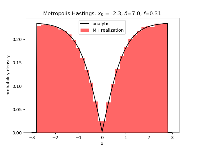
Case 1 – $f_1(x) = |tanh(x)|/N_1$
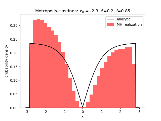
This distribution was chosen since it has a sharp cusp in the center and two fairly flat and broad wings. The best results came from a starting point $x_0 = -2.3$ over in the left wing (the right wing also worked equally well) and a fairly large value of $\delta=7.0$ was chosen such that $f \approx 1/3$. The agreement is quite good.
A smaller value of $\delta$ lead to more samples being collected ($f=0.85$) but the realizations couldn’t ‘shake off the memory’ that they started over in the left wing and the results were not very good, although the two-wing structure can still be seen.
Starting off with $x_0 = 0$ resulted in a realization of random numbers that looks far more like the uniform distribution than the distribution we were hunting.

This result persists with smaller values of $\delta$.
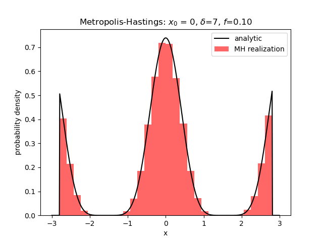
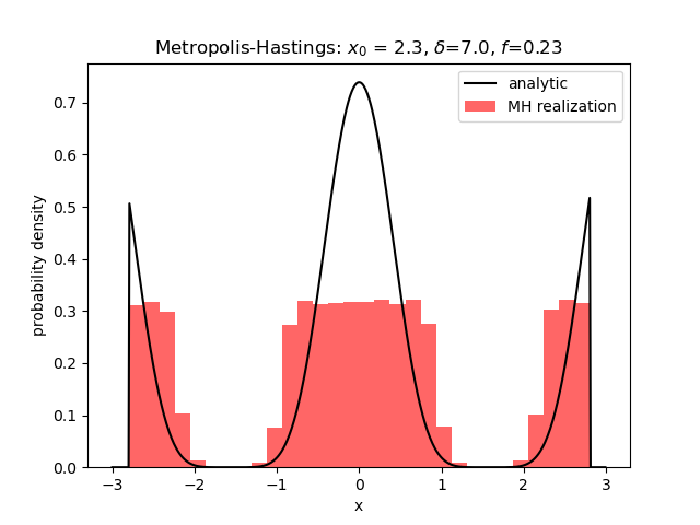
Case 2 – $f_2(x) = \cos^6(x)/N_2$
In this case, the distribution has a large central hump or mode and two truncated wings. The best results came from a starting value of $x_0$ at or near zero and a large value of $\delta$.
Lowering the value of $\delta$ leads to the algorithm being trapped in the central peak with no way to cross into the wings.

Finally, starting in the wings with a large value of $\delta$ leads to a realization that looks like it has the general idea as to the shape of the distribution but without the ability to capture the fine detail.
This behavior persists even when the number of trials is increased by a factor of 10 and no immediately satisfactory explanation exists.