
Neural Networks 1 – Overview
This month’s column begins a new effort that is inspired by and strongly follows the video Building a neural network FROM SCRATCH (no Tensorflow/Pytorch, just numpy & math) by Samson Zhang. Like Zhang, I agree that the best way to learn any algorithm is to build one from scratch even if, and, more important, especially if you are going to use someone else’s code. Usually, one can’t understand the behavior nor appreciate the effort that went into an external package without having ‘walked a mile in another developer’s shoes’. You also don’t know where the algorithm is likely to work or fail if you don’t have some insight into the inner workings.
Zhang provides all of his code and data on his Kaggle notebook and that code base formed the starting point for this exploration. However, the data that were used was from the Kaggle repository by Dariel Dato-On at MNIST in CSV | Kaggle. In both cases the data are derived from the MNIST digitized and labels samples of hand-written numerical digits 0-9, some of which look like:
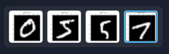
Each image is 28×28 pixels with values ranging from 0-255. For convenience, each image is stored in CSV format as a row consisting of 785 values. The first column contains the label for the image (i.e., ‘0’, ‘5’, ’5’, or ‘7’ for the cases above) and the remaining 784 columns the image data. The entire data set consists of 60,000 such rows. For this first experiment, 59,000 were used as training data and 1,000 as test data to evaluate the success of the net in converging into some useful state.
The basic idea of a neural network is the nonlinear transformation of input arrays to output arrays that provides a high probability of classifying the input data into the correct ‘bucket’. In this example, the input arrays are 784-length, normalized, column vectors with real values ranging $[0,1]$ and the outputs are probabilities of belonging in one of the ten possible output buckets of $[0,1,2,3,4,5,6,7,8,9]$.
Zhang’s network consists of 3-layers: an input layer consisting of 784 slots to accommodate the 784 pixels in each image; a hidden layer consisting of 10 slots, each receiving input from each slot in the previous layer (i.e., input layer), the precise mechanics of which will be discussed below; and finally an output layer consisting of 10 slots, each, again, receiving input from each slot in the previous layer (i.e., the hidden layer). Properly normalized, the values in the output layer can be interpreted as probabilities with the maximum value corresponding to the most likely label.
To be concrete, below is a schematic of how the final trained network decided that a ‘0’ input image should be classified as a ‘0’:
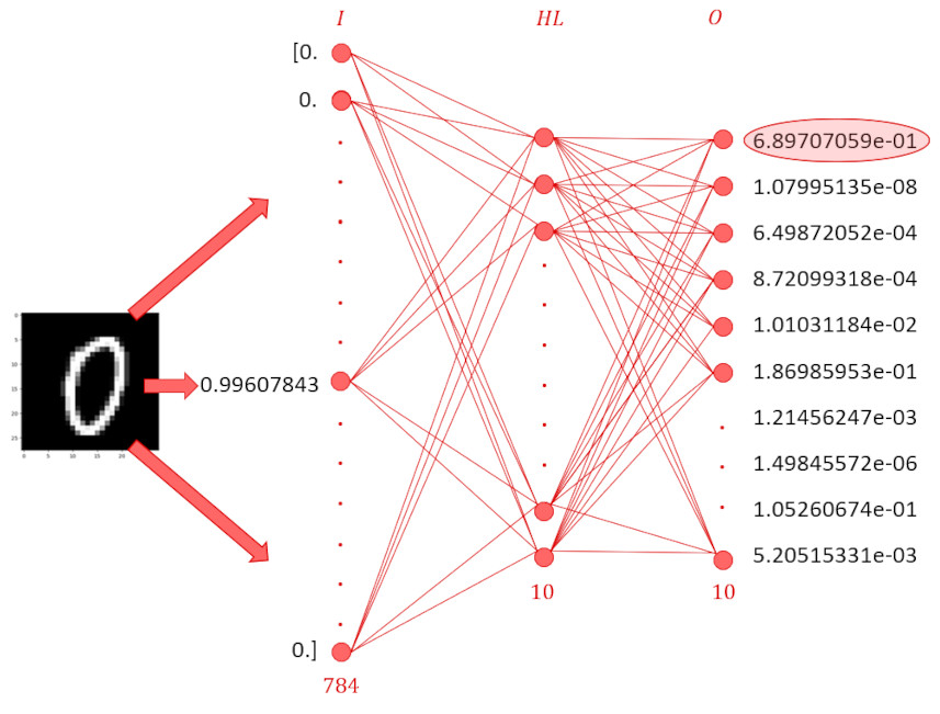
The image of the hand-written ‘0’ was converted to a one-dimensional array with 784 components, four of which are shown being fed into the input layer. Pre-determined weights and biases, $W$ and $b$ at both layers (of different sizes, of course) create an affine transformation of the results of the previous layer
\[ Z^{(1)} = W^{(1)} \cdot X^{(0)} + b^{(1)} \; , \]
where the ‘dot product’ between the $W$ and the $X$ stands for the appropriate matrix product (i.e., $W_{ij} X_{j}$). This transformation is then applied to each image in the training set (Zhang used 39,000 images; the one detailed here used 59,000 – with both cases holding back 1000 images for testing). Typically, for data sets this small, the images are stacked in a single array and fed in all at once since the average cost over the whole set is easily computed with little storage overhead. Thus, there is actually a suppressed index in Zhang’s code. This architecture will be revisited in a latter blog for data sets too large to hold completely in memory but for now Zhang’s approach is followed as closely as possible.
The input, $X^{1}$, for the next layer results from passing these $Z^{(1)}$ outputs through a nonlinear transformation before being passed onto the next layer. The nonlinearity represents the ‘activation’ of each neuron and the current best practice involves using the ReLU function defined as
\[ ReLU(x) = \left\{ \begin{array}{lc} x & x > 0 \\ 0 & {\mathrm otherwise} \end{array} \right. \; , \]
meaning that
\[ X^{(1)} = ReLU(Z^{(1)}) \; . \]
The dimensionality of each column of $Z^{(1)}$ is now 10, although different numbers of neurons in the hidden layer are also possible. This is another point deferred to a later blog.
The transformation from the hidden layer to the output layer works in much the same way with
\[ Z^{(2)} = W^{(2)} \cdot X^{(1)} + b^{(2)} \; , \]
but the nonlinear transformation to the output layer is, in this case, the SoftMax transformation that normalizes the each of the nodes on the output layer against the whole set using
\[ X^{(2)} = \frac{\exp(Z^{(2)})}{\sum \exp(Z^{(2)})} \; , \]
resulting in a functional form reminiscent, up to the sign of the exponent, of the partition function from statistical mechanics.
Of course, the classification ability of the neural network will be poor for a set of arbitrary weights and biases. The key element in training the net is to find a combination of these values that maximizes the performance of the net across the statistically available input – in other words, an optimization problem.
In the lingo of neural nets, this optimization problem is solved via the back-propagation process, which basically depends on the differentiability of the transformations and the implicit (or inverse) function theorems to determine the proper inputs given the desired outputs. The starting point is the formation of the ‘residuals’ $R$ (a term used locally here) defined as
\[ R = X^{(2)} – Y \; , \]
where $Y$ is the true or correct value for the labeled image. For the ‘0’ example above, $Y$ will look like the 10-element array
\[ Y = \left[ 1, 0, 0, 0, 0, 0, 0, 0, 0, 0 \right] \; .\]
If the label had been ‘4’, then the 1 would have been put in the corresponding spot for four, which is the fifth array element in from the left.
The equations Zhang cites for this back propagation:
\[ dZ^{[2]} = A^{[2]} – Y \; , \]
\[ dW^{[2]} = \frac{1}{m} dZ^{[2]} A^{[1]T} \; ,\]
\[ dB^{[2]} = \frac{1}{m} \Sigma {dZ^{[2]}} \; , \]
\[dZ^{[1]} = W^{[2]T} dZ^{[2]} .* g^{[1]\prime} (z^{[1]}) \; ,\]
\[ dW^{[1]} = \frac{1}{m} dZ^{[1]} A^{[0]T} \; ,\]
and
\[ dB^{[1]} = \frac{1}{m} \Sigma {dZ^{[1]}} \; .\]
These equations clearly show the backwards chaining of derivatives via the chain rule but are quite difficult to decode as he mixes notation (for example his $A$’s are also $X$’s) and intermixes some of the broadcasting rules he uses when employing numpy (hence the factor of $m$, which is the size of the number of rows in the training data set and the presence of the transposed $T$ notation) with those representing the connecting edges of the net. Nonetheless, his code for the net works reasonably well with an achieved accuracy of about 85% to 89% on the test set and it forms an excellent starting point for building a neural network from the ground up.
Next month’s blog will focus on coding the nuts and bolts of a similar network from scratch with along with a proper derivation of the back propagation.