
Visions of Clustering
In a column from a few months ago (Fooling a Neural Network), I discussed the fact that human beings, regardless of mental acuity, background, or education, see the world in a fundamentally different way than neural networks do. Somehow, we are able to perceive the entire two-dimensional structure of an image (ignoring for the time being the stereoscopic nature of our vision that leads to depth perception) mostly independent of the size, orientation, coloring, and lighting. This month’s column adds another example of the remarkable capabilities of human vision when compared to a computer ‘vision’ algorithm in the form of an old algorithm with a new classification.
The Hoshen-Kopelman algorithm was introduced by Joseph Hoshen and Raoul Kopelman in their 1976 paper Percolation and Cluster Distribution. I. Cluster Multiple Labeling Technique and Critical Concentration Algorithm. The original intent of the algorithm was to identify and label linked clusters of cells on a computational grid as a way of finding spanning clusters in the percolation problem. A spanning cluster is a set of contiguous cells with orthogonal nearest neighbor that reach from one boundary to the opposite side. The following image shows a computational 7×7 grid where the blue squares represent an occupied site and the white squares as vacant ones. Within this grid is a spanning cluster with 24 linked cells that reaches from the bottom of the grid to the top and which also spans the left side of the grid to the right.
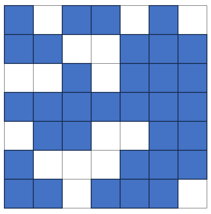
The original intention of percolation models was to study physical systems such as fluid flow through irregular porous materials like rock or the electrical conduction of random arrangement of metals in an insulating matrix. But clearly the subject has broader applicability to various problems where the connection topology of a system of things is of interest such as a computer network or board games. In fact, the configuration shown above would be a desirable one for the charming two-player game The Legend of Landlock.
Now the human eye, beholding the configuration above has no problem finding, with a few moments of study, that there are 4 distinct clusters: the large 24-cell one just discussed plus two 3-cell, ‘L’-shaped ones in the upper- and lower-left corners and a 2-cell straight one along the top row. This is a simple task to accomplish for almost anyone older than a toddler.
Perhaps surprisingly, ‘teaching a machine’ (yes this old algorithm is now classified – at least according to Wikipedia – as a machine learning algorithm) to identify clusters like these is a relatively complicated undertaking requiring rigorous analysis and tedious bookkeeping. The reasons for this speak volumes for how human visual perception differs sharply from machine vision. However, once the machine is taught to find clusters and label them, it tirelessly and rapidly tackles problems humans would find boring and painful.
To understand how the algorithm works and to more clearly see how it differs essentially from how humans perform the same task, we follow the presentation of Harvey Gould and Jan Tobochnik from their book An Introduction to Computer Simulation Methods: Applications to Physical Systems – Part 2. The grid shown above is taken from their example in Section 12.3 cluster labeling (with some minor modifications to suit more modern approaches using Python and Jupyter).
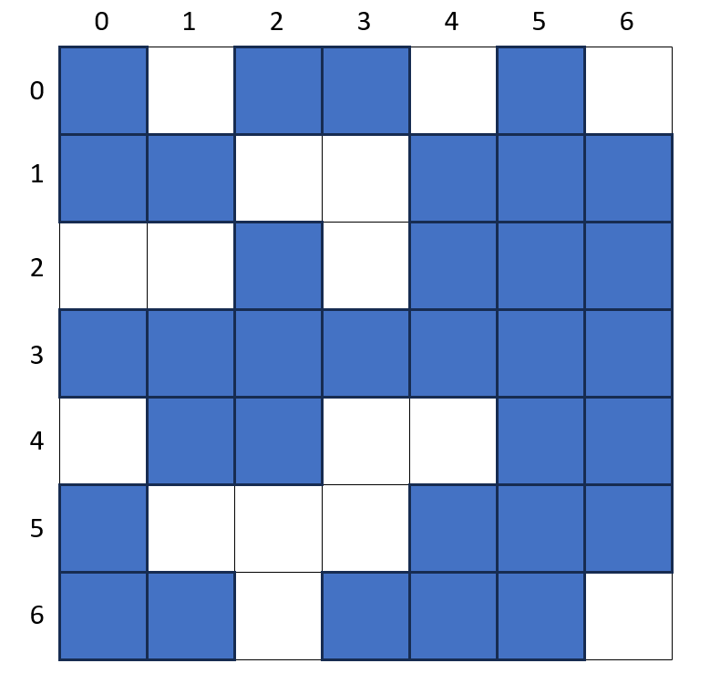
Assuming that the grid is held in a common 2-dimensional data structure, such as a numpy array, we can decorate the lattice with row and column labels that facilitate finding a grid cell.
We start our cluster labeling at 1 and we use a cluster labeling variable to keep track of the next available label when the current one is assigned. The algorithm starts in the cell in the upper left corner and works its way, row by row, across and down, looking at cells immediately up and left to see if the current on is linked to cells in the previous row or column. This local scanning may seem simple enough but generically there will be linkages later on that coalesce two distinct clusters into a new, larger, single cluster and this possibility is where the subtly arises. This will become much clearer as we work through the example.
Since the cell at grid (0,0) is occupied, it is given the label of ‘1’ and the cluster label variable is incremented to ‘2’. The algorithm then moves to cell (0,1). Looking left is finds that the current cell is occupied and that it has a neighbor to the left and so it too is labeled with a cluster label ‘1’. The scan progresses across and down the grid until we get to cell (1,5).
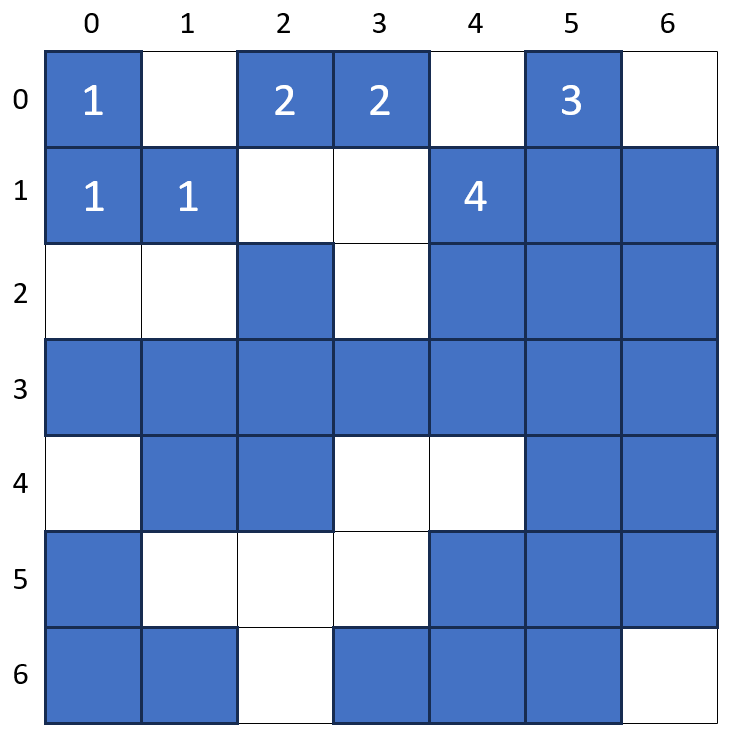
Note that at this point, the human eye clearly sees that the cells at (1,4) and (1,5) are linked neighbors and that the assignment of the cluster label ‘4’ to cell (1,4) was superfluous since it really is a member of the cluster with label ‘3’ but the computer isn’t able to see globally.
The best we can do with the machine is to locally detect when this happens and keep a ‘second set of books’ in the form of an array that lets the algorithm know that cluster label ‘4’ is really a ‘3’. Gould and Tobochnik call the cluster label ‘4’ as improper and the label ‘3’ as proper but raw and proper are better terms.
When the algorithm has finished scanning the entire grid, the raw cluster labels stand as shown in the following image.
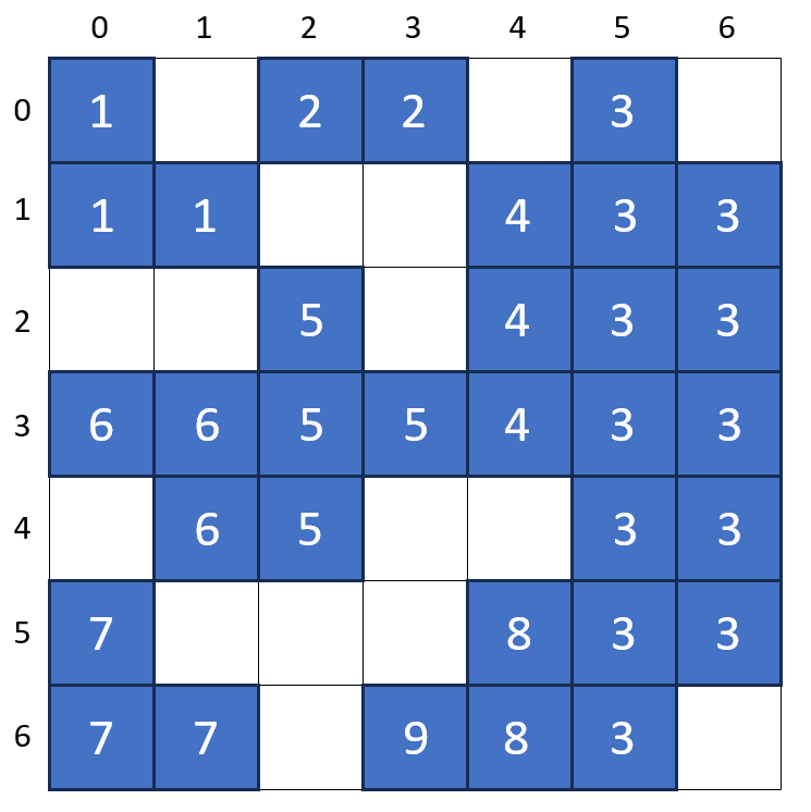
Note that the largest cluster label assigned is ‘9’ even though there are only 4 clusters. The association between the raw labels and the proper ones is given by:
{1: 1, 2: 2, 3: 3, 4: 3, 5: 3, 6: 3, 7: 7, 8: 3, 9: 3}
Any raw labels that are identical with their proper labels are distinct and proper with no additional work. Those raw labels that are larger in value than their proper labels are part of the cluster with the smaller label. The final step for this example is cosmetic and involves relabeling the raw labels ‘4’, ‘5’, ‘6’, ‘8’, and ‘9’ as ‘3’ and then renumbering the ‘7’ label as ‘4’. All of this is done with some appropriate lookup tables.
One thing to note. Because ‘8’ linked to ‘3’ in row 5, ‘8’ had 3 as a proper label before ‘9’ linked to ‘8’ and thus, when that linkage was discovered, the algorithm code immediately assigned a proper label of ‘3’ to ‘9’. Sometimes the linkages can be multiple layers deep.
Consider the following example.
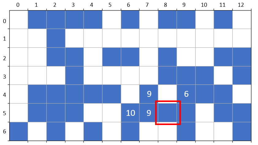
By the time the algorithm has reached cell (5,8) it has assigned cluster label ‘10’ to cell (5,6) but has associated with it a proper label of ‘9’ based its subsequent discovery in cell (5,7). Only when the machine visits cell (5,8) does it discover that cluster label ‘9’ is no longer proper and should now be associated with the proper label ‘6’. Of course, the algorithm ‘knows’ this indirectly in that it has the raw label ‘10’ associated with the label ‘9’ which is now associated with the proper label ‘6’. Thus the association between raw and proper labels is now a two-deep tree given by (key part highlighted in red):
{1: 1, 2: 2, 3: 3, 4: 4, 5: 5, 6: 6, 7: 7, 8: 1, 9: 6, 10: 9, 11: 11, 12: 12}
Again, a human being simply doesn’t need to go through these machinations (at least not consciously) further emphasizing the gap between artificial intelligence and the real one we all possess.
(Code for my implementation of the Hoshen-Kopelman algorithm in python can be found in the Kaggle notebook here.)