
Time Series 4 – Introduction to Kalman Filtering
This month we turn from the exponential smoothing and moving average techniques for analyzing time series and start a sustained look at the Kalman filter. The Kalman filter has been hailed as one of the most significant mathematical algorithms of the 20th century. The primary reason for this praise is that the Kalman filtering enables a real time agent to make mathematically precise and supported estimates of some quantity as each data point comes in rather than having to wait until all the data have been collected. This enabling behavior garners Kalman filtering a lot of attention and Russell and Norvig devote part of their chapter on probabilistic reasoning in their textbook Artificial Intelligence: A Modern Approach to it.
Before diving into the mathematical details, it is worth noting that the thing that sets the Kalman filter apart from the Holt-Winters algorithm is that in the latter, we needed to recognize and characterize a reoccurring pattern in our data. For example, in the Red Fin housing sales, the data are conveniently regularly spaced in monthly intervals and seasonal patterns are readily apparent if not always predictable. The Kalman filter imposes no such requirements, hence its usefulness. It is often used in navigation activities within the aerospace field where it is applied to powered flight of a missile as readily as to a low-Earth orbiting spacecraft like Starlink to a libration orbiting spacecraft like JWST.
There are an enormous number of introductions to the Kalman filter each of them with their own specific strengths and weakness. I tend to draw on two works: An Introduction to the Kalman Filter by Greg Welch and Gary Bishop and Poor Man’s Explanation of Kalman Filtering or How I stopped Worrying and Learned to Love Matrix Inversion by Roger M. du Plessis. The latter work is particularly difficult to come by, but I’ve had it around for decades. That said, I also draw on a variety of other references which will be noted when used.
I suppose there are four core mathematical concepts in the Kalman filter: 1) the state of the system can be represented by a list of physically meaningful quantities, 2) these quantities vary or evolve in time in some mathematically describable way, 3) some combination (often nonlinear) of the state variables may be measured, 4) the state variables and the measurements of them are ‘noisy’.
Welch and Bishop describe these four mathematical concepts as follows. The state, which is described by a $n$-dimensional, real array of variables
\[ x \in \mathbb{R}^n \; \]
evolves according to the linear stochastic differential equation
\[ x_k = A x_{k-1} + B u_{k-1} + w_{k-1} \; , \]
where $A$, which is known as the $n \times n$ real-valued process matrix, provides the natural time evolution of the state at earlier time $t = k-1$ to the state at time $t = k$. The quantity $u \in \mathbb{R}^{\ell} $ is a control or forcing term that is absent in the natural dynamics but can be impose externally on the system. The $n \times \ell$, real-valued matrix $B$ maps the controls into the state evolution. The term $w \in \mathbb{R}^n$ is the noise in the dynamics; it typically represents those parts of the natural evolution or of the control that are either not easily modeled or are unknown.
Measurement of the state is represented an $m$-dimensional, real-valued vector $z \in \mathbb{R}^m$ and is related to the state by the equation
\[ z_k = H x_k + v_k \; , \]
where $H$ is a $m \times n$ real-valued matrix and $v \in \mathbb{R}^m$ is the noise in the measurement.
In addition, both noise terms are assumed to be normally distributed with their probabilities described by
\[ p(w_k) = N(0,Q_k) \; \]
and
\[ p(v_k) = N(0,R_k) \; , \]
where $Q_k \in \mathbb{R}^{n \times n}$ is the process noise covariance matrix and $R_k \in \mathbb{R}^{m \times m}$ is the measurement noise covariance matrix. We further assume that they are uncorrelated with each other. Generally, these noise covariances are time-varying since their values typically depend on the state.
Note that both the state and measurement equations are linear. More often than not, Kalman filtering is applied to nonlinear systems but in those cases, the estimation process is linearized and the above equations are used. Whether that is a good idea or not is a discussion for another day.
The role of the Kalman filter is to produce the best estimate of the state at a given time given the above equations. To do so, the filter algorithm draws heavily on concepts from Bayesian statistics to produce a maximum likelihood estimate.
In terms of Bayesian statistics, the algorithm assumes both an a priori state estimate ${\hat x}^{-}_{k}$ and an a posteriori one ${\hat x}_{k}$. The transition from the a priori to the a posteriori is made with
\[ {\hat x}_k = {\hat x}^{-}_{k} + K_k (z_k – H {\hat x}^{-}_k ) \; , \]
where the ‘magic’ all happens due to the Kalman gain $K_k$ defined as
\[ K_k = P^{-}_k H^T \left( H P^{-}_k H^T + R \right) ^{-1} \; , \]
where ‘$T$’ indicates a matrix transpose.
Note that this equation is functionally similar to the running average form calculated as
\[ {\bar x} = {\bar x}^{-} + \frac{1}{N} \left( x_N – {\bar x}^{-} \right) \; . \]
We’ll return to that similarity in a future post.
For now, we will round out the menagerie of mathematical beasts by noting that $P_k$ is the state covariance, a $n \times n$, real-valued matrix, that summarizes the current statistical uncertainty in the state estimation. Formally, it is defined as
\[ P_k = E \left[ (x_k – {\hat x}_k ) (x_k – {\hat x}_k )^T \right] \; , \]
where the ‘$E$’ stands for expectation over the state distribution.
The state covariance can be associated with the a priori estimate, where it is denoted as $P^{-}_k$ or with the a posteriori estimate, where it is denoted by $P_k$. The two are related to each other by
\[ P_k = A P^{-}_k A^T + Q \; . \]
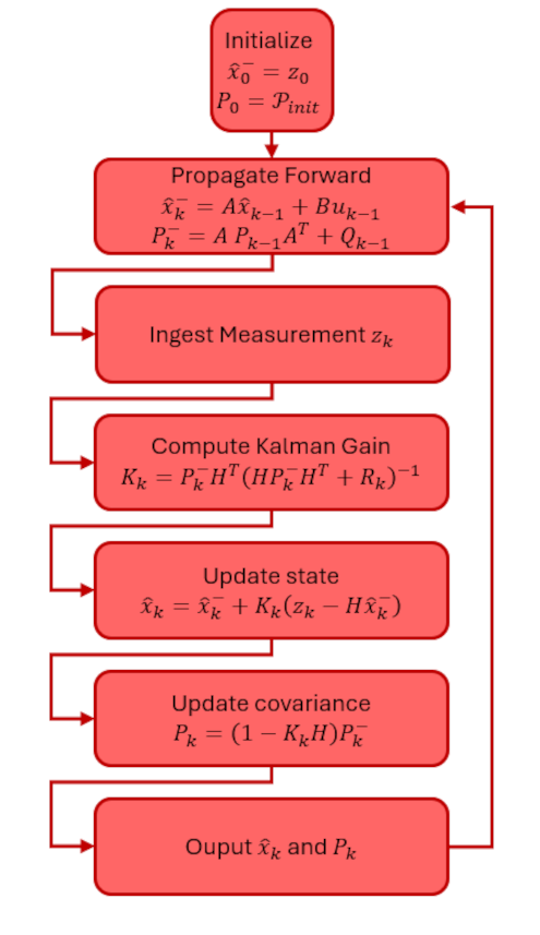
The Kalman algorithm is best summarized using the following flow diagram adapted from the one in Introduction to Random Signals and Applies Kalman Filtering 4th Edition by Brown and Hwang.
In future blogs, we’ll explore how to derive the magical Kalman gain, some applications of it to agent-based time series estimation, and a variety of related topics. It is worth noting that the notation is fluid, differing from author to author and application to application.