Time Series 6 – Recursive Least Squares
The last post introduced the notion of the recursive least squares estimation approach as a natural precursor to the Kalman filter and derived the Kalman-like gain that governed the state estimation update equation. Before moving on to a simple example of the Kalman filter, it seemed prudent to show the recursive least squares filter in action with a numerical example.
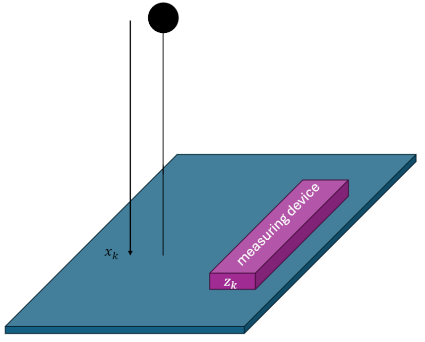
The example involves a mass falling in an unknown uniform gravitational field with unknown initial conditions. At regular time intervals, a measurement device measures the height of the mass above the ground but only to within certain precision due to inherent noise in it measuring processes. The challenge is then to deliver the best estimate of the unknowns (initial height, initial speed, and the uniform gravitational acceleration). We will assume that, beyond a measurement of the initial height, the other initial conditions are inaccessible to the measurement device since it only measures range. This example is adapted from the excellent article Introduction to Kalman Filter: Derivation of the Recursive Least Squares Method by Aleksander Haber.

To prove that the recursive least squares method does generate a real least squares estimation, let’s first look at how a batch least squares approach to this problem would be performed.
The dynamics of the falling mass are given by
\[ d(t) = d_0 + v_0 t + \frac{1}{2} a t^2 \; , \]
where $d(t)$ is the height above the ground at a given instant.
We assume that the above equation is exact; in other words, there are no unknown forces in the problem. In the language of Kalman-filtering and related optimal estimation, there is said to be no process noise, with it understood that the word ‘process’ is a genetic umbrella meaning the dynamics by which the state evolves in time, for which Newton’s laws are an important subset.
By design, measurements come in every $\Delta t$ seconds and so the time evolution of the fall of the mass is sampled at times $t_k = k \Delta t$. At measurement time $t_k$ the amount the mass has dropped is
\[ x_k = x_0 + v_0 k \Delta t + \frac{1}{2} k^2 \Delta t^2 a \; \]
and the corresponding measurement is
\[ z_k = x_k + \eta_k \; , \]
where $\eta_k$ is the noise the measuring device introduces in performing its job.

The batch least squares estimation begins by writing the evolution equation in a matrix form
\[ z_k = \left[ \begin{array}{ccc} 1 & k \Delta t & \frac{1}{2} k^2 \Delta t^2 \end{array} \right] \left[ \begin{array}{c} x_0 \\ v_0 \\ a \end{array} \right] + \eta_k \equiv H_{k,p} x_p + \eta_k \; . \]
The array $x_p$ contains the constant initial conditions and unknown acceleration that is being estimated.
For this numerical experiment, $x_0 = -4m$, $v_0 = 2 m/s$ (positive being downward), and $a = 9.8 m/s^2$ the usual value for surface of the Earth (give or take regional variations). Measurements are taken every $\Delta t = 1/150 s$ over a time span of 14.2 seconds. To illustrate the meaning of $H_{k,p}$, the value of the matrix at $k=0$ is
\[ H_{k=0,p} = \left[ \begin{array}{ccc} 1 & 0 & 0 \end{array} \right] \; \]
corresponding to an elapsed time of $t_k = 0$ and at $k = 75$
\[ H_{k=0,p} = \left[ \begin{array}{ccc} 1 & 0.5 & 0.125 \end{array} \right] \; \]
corresponding to an elapsed time of $t_k = 0.5$.
The merit of this matrix approach is that by putting every measurement into a batch we can write the entire measured dynamics in a single equation as:
\[ z = H x + \eta \; . \]
The array $z$ has $M$ elements (for the number of measurement), where $M$ is the maximum value of the time index $k$ (for this specific example $M$ = 2131). The matrix $H$ is a $M \times n$ where $n$ is the number of estimate parameters ($n$ = 3, in this case) and $x$ is the array of parameters to be estimated). The array $\eta$ represents the $M$ values of random noise (assumed to be stationary) that were present in the measurements. The values of $\eta$ used in this numerical example were drawn from a normal distribution with a zero mean and a standard deviation of 1; the latter value determines the value of $R_k = 1$.
Since, in the matrix equation above, the matrix $H$ isn’t square, it may not be obvious how to solve for $x$. However, there is a well-known technique using what is known as the Moore-Penrose pseudoinverse.
In short, to solve for $x$ in a least squares sense, we set $\eta$ to zero (i.e., we ignore the noise assuming the classical argument that with enough measurements the influence of the noise will average to zero). We then left-multiply by the transpose of $H$ to get
\[ H^T z = (H^T H) x \; .\]
The quantity $H^T H$ is a $(n \times K) \cdot (K \times n) = n \times n $ matrix (in this case $3\times 3$, which is invertible. We then arrive at the compact form of the estimate for $x$ as
\[ x_{est} = (H^T H)^{-1} H^T z \; .\]
For this numerical experiment, the resulting estimate is
\[ x_{est} = \left[ \begin{array}{c} -3.95187658 \\ 1.99300377 \\ 9.80040125 \end{array} \right] \; .\]
This is the same value one gets by using a package like numpy’s linalg.lstsq.
In the recursive method, all of the data are not stored and handled at once but rather each point is taken and processed as it comes in.
The algorithm developed in the last post is summarized as:
- Start each step with the current time $t_k$, measurement $z_k$, and the previous estimates of the state $x_{k-1}$ and the covariance $P_{k-1}$
- Perform the $k$-th calculation of the gain: $K_k = P_{k-1} \cdot H_k^T \cdot S_k^{-1}$, where $S_k = H_k \cdot P_{k-1} \cdot H_k^T + R_k$
- Make the $k$-th estimate of the unknowns: ${\hat x}_k = {\hat x}_{k-1} + K_k \left( z_k – H_k {\hat x}_{k-1} \right)$
- Make the $k$-th update of the covariance matrix: $P_k = \left(I – K_k H_k \right)P_{k-1} $
Using this algorithm, the time evolution of the estimated initial position is

with a final value of -3.95170034.
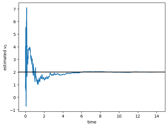
Likewise, the time evolution of the estimated initial speed is

with a final value of 1.99295453.
And, finally, the time evolution of the estimated acceleration is

with a final value of 9.80040698.
These estimated values, up to the numerical noise introduced by a different set of floating point operations, are identical with the batch least squares numbers.
