
A Symbolic Experiment – Part 7: Derivative Rewriting
With all of the elementary ingredients for term rewriting for generic expressions in Sympy in hand, we now turn to a specialized but important corner: rewriting expressions involving a derivative. What we specifically want to do is to implement the Fourier differentiation rule
\[ {\mathcal F} \left[ \frac{d^n f(t)}{d t^n} \right] = (i \omega)^n F(\omega) \; ,\]
where the two functions $f(t)$ and $F(\omega)$ are members of a Fourier transform pair.
The steps involved here are a bit different in than the earlier term rewriting rules covered because even the simplest derivative is a complex expression involving a function, its arguments, the notion of a limit ratio, the number of times a derivative is to be taken (i.e., the value of $n$ in the formula above), and what terms are kept constant.
For instance, the expression
\[ \frac{d}{dx} f(x) \; \]
has the tree representation of
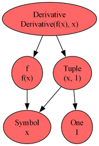
where the value of $n$ is held in the Sympy Tuple $(x,1)$, which is a specialized Sympy container designer to look like a conventional Tuple but whose elements are limited to Sympy objects. Likewise the expression
\[ \frac{\partial^3}{\partial y^2 \partial x} h(x,y) \; \]
corresponds to the following tree diagram
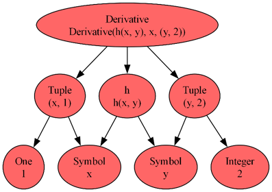
Note that there are two instances of the Sympy Tuple to hold the number of derivatives with respect to $x$ and $y$ separately.
With so many moving pieces it shouldn’t come as a surprise that the Derivative objects in Sympy come equipped with a few extra functions. The ones we will need to implement the Fourier derivative rule are:
- .derivative_count – counts the number of times a derivative operator is applied regardless of the variable. Returns 1 for the first expression above and 3 for the second.
- .variable_count – returns a tuple (not a Sympy Tuple) containing the instances of Sympy Tuple used in the expression. Returns $(x,1)$ for the first expression above and $(y,2)$ for the second.
- .variables – returns a tuple (not a Sympy Tuple) containing the variables used in the differentiation, repeated as specified in .variable count. Returns $(x,)$ for the first expression above and $(x,y,y)$ for the second. Variables that are not involved in the Derivative are treated as constants and do not show up (although they will still show up in .args or .atoms())
The key term rewriting function is .replace() and, as alluded to in the end of the previous post, we will be passing anonymous lambda functions to it.
To better understand why this is the proper method of attack, we can look at what .replace actually does. The following is an adaptation of Sympy’s own documentation on .replace and the Stack Overflow discussion Sympy subs vs replace vs xreplace. The proper pattern of the .replace function is:
.replace(query, value, map=False, simultaneous=True, exact=None)
As .replace walks across the expression tree at each node it runs the provided query. If that application of query returns true then that particular node will be replaced with the provided value. Our strategy will be to make two passes over the expression tree:
- In the first pass, we will query if the node is of type Derivative. If it is we will make the substitution that $\frac{d^n}{dt^n} f(t) \rightarrow (i t)^n f(t)$.
- In the second pass, we will replace each instance of $t$ by $\omega$ and each instance of $f$ with $F$.
Pass 1
For Pass 1, the query is given by the lambda function:
is_deriv = lambda e: isinstance(e, sym.Derivative)
The value is a bit more involved and is given by
val = lambda e: sym.Mul(e.expr, *[sym.I*v for v,n in e.variable_count for _ in range(n)])
To understand this code, lets look at the related list comprehension
[v for v,n in e.variable_count for _ in range(n)]
This list comprehension is basically a nested for loop. The outer loop unpacks the expression e’s .variable_count tuple into the two variables v and n while the inner loop writes v’s value n times in the list. For the first expression above the resulting list is [$x$] while it is [$x$,$y$,$y$] for the second one.
The actual list comprehension used in the value portion of .replace multiplies each term by $i=\sqrt{-1}$, giving the lists [$ix$] and [$ix$,$iy$,$iy$] for the first and second expressions above. The splat/unpacking operator ‘*’ removes the list container making the arguments acceptable to Mul.
In symbolic form, the value transforms
\[ \frac{d}{dx} f(x) \rightarrow \imath x f(x) \; \]
and
\[ \frac{\partial^3}{\partial y^2 \partial x} h(x,y) \rightarrow -\imath x y^2 h(x,y) \; .\]
Pass 2
For Pass 2, the elementary term rewriting rules discussed in the previous post can be followed without any difficulty by using .subs with a dictionary that maps variable and function pairings to each other.
def Fderiv_subs(expr,pairs): temp1 = expr.replace(is_deriv,val) return temp1.subs(pairs)
For the first expression, suppose we Fourier pair $t$ and $\omega$ and $f$ and $F$, then the invocation
simp1 = sym.diff(f(t),t)
simp1 = sym.diff(f(t),t) display(Fderiv_subs(simp1,{t:w,f:F}))
gives the desired transformation
\[ \frac{d}{dt} f(t) \rightarrow \imath \omega F(\omega) \; .\]
With a bit more generalization more complex Fourier pairings can also be accommodated.
In the next post, we’ll put all these pieces together to complete the Fourier term rewriting project embarked upon at the beginning of this series.