Monthly Archive: March 2016

It’s a rare thing to find a clear and simple explanation for something complicated – something like the Pythagorean Theorem or calculus or whatnot.  It’s even rarer to find a clear and simple explanation for something that challenges the very pillars of logic – something like Gödel’s Theorem or the halting theorem.  But J. Glenn Brookshear treats readers of his text Computer Science: An Overview to a remarkably clear exploration of the halting theorem in just a scant 3 pages in Chapter 12. I found this explanation so easy to digest that I thought I would devote a post to it, expanding on it in certain spots and putting my own spin on it.

Now to manage some expectations:  it is important to note that this proof is not rigorous; many technical details needed to precisely define terms are swept under the rug; but neither is it incorrect.  It is logically sound if a bit on the heuristic side.

The halting theorem is important in computer science and logic because it proves that it is impossible to construct an algorithm that is able to analyze an arbitrary computer program and all its possible inputs and determine if the program will run to a successful completion (i.e. halt) or will run forever, being unable to reach a solution.  The implications of this theorem are profound since its proof demonstrates that some functions are not computable and I’ve discussed some of these notions in previous posts.  This will be the first time I’ve set down a general notion of its proof.

The basic elements of the proof are a universal programing language, which Brookshear calls Bare Bones, and the basic idea of self-referential analysis.

The Bare Bones language is a sort of universal pseudocode to express those computable functions that run on a Turing Machine (called Turing-computable functions).  The language, which is very simple, has three assignment commands:

• Clear a variable
• Increment a variable
• Decrement a variable

In addition, there is one looping construct based on the while loop that looks like

while x not 0 do;
   ...
end;

While primitive, these commands make it possible to produce any type of higher level function.  For  example, Brookshear provides an algorithm for computing the product of two positive integers:

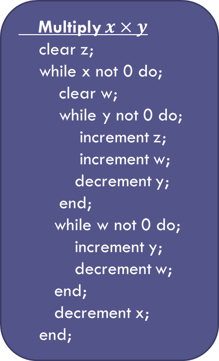
Note: for simplicity only positive integers will be discussed – but the results generalize to any type of computer word (float, sign int, etc.).

Now Bare Bones is a universal language in the sense that researchers have demonstrated that all Turing-computable functions can be expressed as Bare Bones algorithms similar to the Multiply function shown above.  Assuming the Church-Turing thesis, which states that the set of all computable functions is the same as the set of all Turing-computable functions, allows one to conclude that Bare Bones is sufficiently rich to encode all algorithms that express computable functions.

One particularly important Bare Bones algorithm is something I call x-test (since Brookshear doesn’t give it a name).

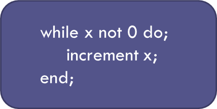
The job of x-test is simple: it either terminates when x is identically zero or it runs forever otherwise.

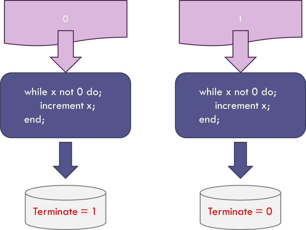
The Terminate flag is assigned a value of 0 if x-test fails to halt and 1 if it does.

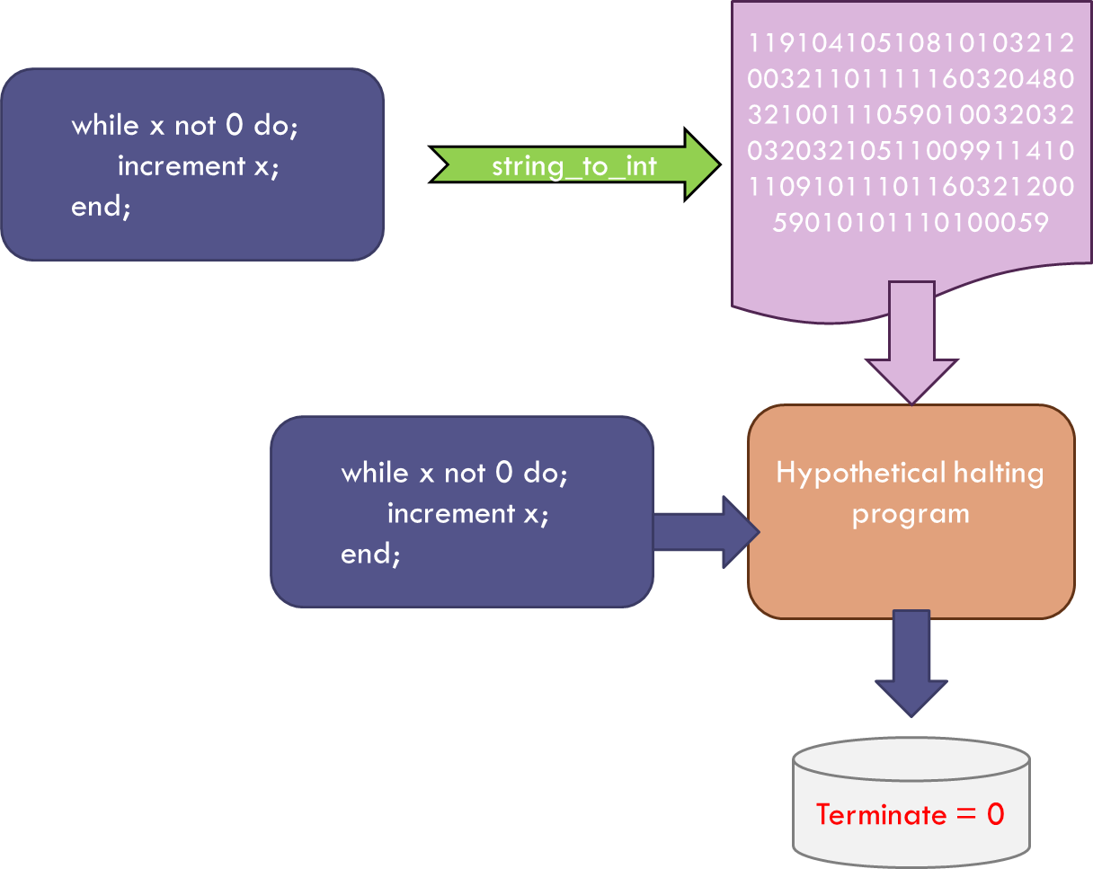
The next step brings in the concept of self-reference.  The function x-test takes an arbitrary integer in and gives the binary output or 0 or 1.  Since x-test is expressed as a set of characters in Bare Bones and since each character can be associated with an integer, the entire expression of x-test can be associated with an integer.  To be concrete, the string representation of x-test is:

‘while x not 0 do;\n    increment x;\nend;’

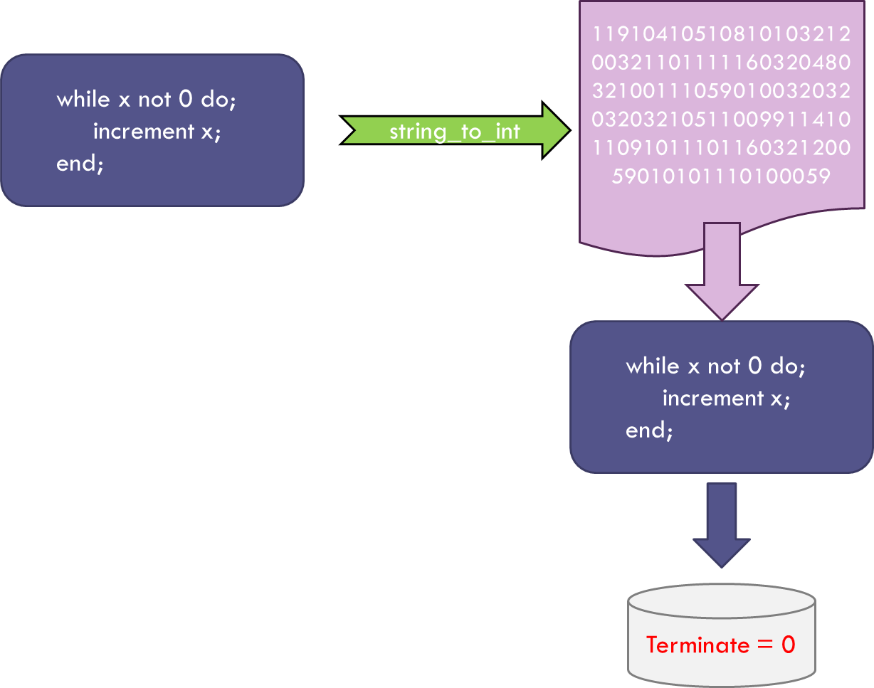
A simple python program, called string_to_int:

def string_to_int(s):
    ord3 = lambda x : '%.3d' % ord(x)
    return int(''.join(map(ord3, s)))

transforms this string to the (very long) integer

119104105108101032120032110111116032048032100111059010032032032032105110099114101109101110116032120059010101110100059

Using this integer in x-test results in the Terminate flag equal 0.

Of course, any expression of x-test in any programming language will result in a nonzero integer and so x-test never has a chance to terminate.

But there are clearly functions that do terminate when they are expressed as input for their own execution (one obvious example is the duel function to x-test where the while loop stops if x is non-zero).  Such functions are said to be self-terminating.

Although it may look like a lot of effort for nothing, this notion of self-terminating functions is the key to the halting theorem and all that remains is to combine the above results with some clever thinking.

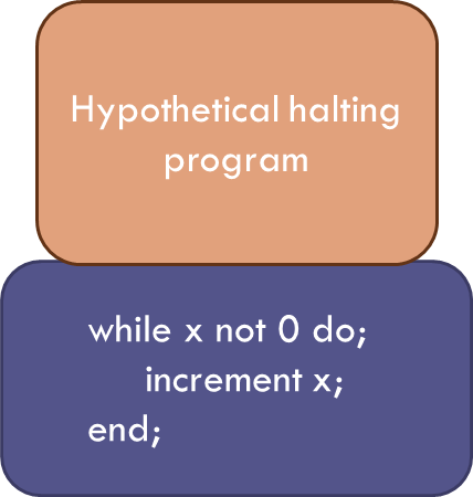
The clever thinking starts with the assumption that there exists a function, which I call the Hypothetical Halting Program (HHP), that can analyze any arbitrary program written in Bare Bones along with any corresponding input and determine which combinations will terminate (decidable) and which will not (undecidable).

Again, to be concrete, let’s look at what the HHP would do when looking to see if x-test is self-terminating.

The HHP would be given the x-test function and the corresponding input (x-test in integer form) and would determine, just as we did above, that x-test won’t terminate – that is, x-test is not self-terminating.

Now such a function that works only on x-test is easy to understand; the text above that argued against x-test being self-terminating is one such instantiation.  However, the goal is to have the HHP be abale to analyze all such algorithms so that we don’t have to think.  Already, warning bells should be going off, since the word ‘all’ is a pretty big set, in fact infinite, and infinite sets have a habit of behaving badly.

But let’s set aside that concern for the moment and just continue our assumption that HHP can do the job.  As we progress, we’ll see that our assumption of the existence of the HHP will lead to a contradiction that rules out this assumption and, thus, gives the desired proof.  Operating without this foresight, we argue that since the HHP is computable it must be able to find expression as a Bare Bones program.  And since the HHP analyzes Bare Bones programs, it must be able to analyze itself and determine if it is self-terminating – spitting out a 1 if so and a 0 otherwise.

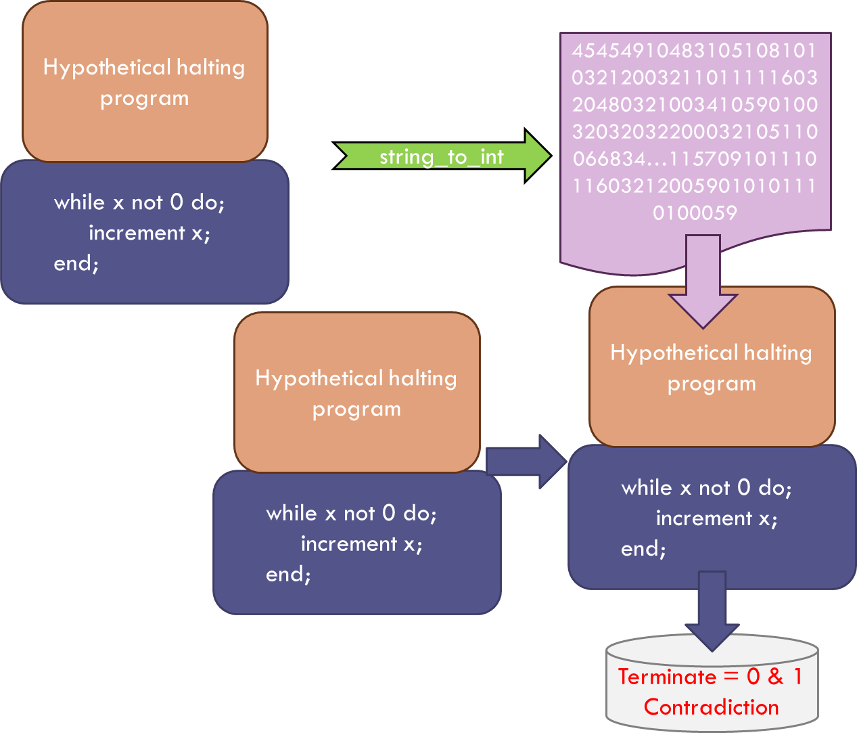
Now we can construct a new program, called the HHP++, that is the sequential running of the HHP followed by x-test.

We can always do this in Bare Bones by first running HHP and then assigning its output (0 or 1) to the input of x-test.  And here is where it gets interesting.

Take the HHP++ and let it test itself to see if it is self-terminating.  If it is self-terminating, the HHP piece will confirm it so and will output a value of 1.  This value is then passed to the x-test piece which then falls to halt.  If the HHP++ is not self-terminating, the HHP piece will output a 0 which, when passed to the x-test piece, halts the operation.  Thus the HHP++ is a program that is neither self-terminating nor not self-terminating and so the only way that can be true is that our original assumption that the HHP exists is false.

It is remarkable that using such a simple argument, the human mind is able to rule out the possibility of general function like the HHP.

For many of us, it’s hard to imagine how the standard blackboard construction of lines and points in the plane can hold any mystery or subtlety. What could be simpler than drawing a line in two dimensions and decorating it with some points, each bearing a label? However, many of the intuitive notions that we have about things aren’t sufficiently well-defined to survive the transition from casual use to rigorous proof. This is especially true in all things associated with getting a computer to perform a set of functions for us; the first step in building good software often being the sharpening of fuzzy ideas. The human capacity to ‘figure it out’ has yet to be designed into a set of instructions.

The issue that arises in constructing a line with points in the plane is in understanding the distinction between the ordered pair of numbers used to denote a given point and the ordered pair of numbers used to denote a vector. Take the line $\ell$ in the plane.

The points ${\mathcal P}$ and ${\mathcal Q}$ fall on the line and have coordinates given by the ordered pairs

\[ {\mathcal P} = \left( \begin{array}{c} x_1 \\ y_1 \end{array} \right) \]

and

\[ {\mathcal Q} = \left( \begin{array}{c} x_0 \\ y_0 \end{array} \right) \; . \]

Note that there is nothing special about writing the points in terms of column arrays, rather than the more usual $(x_i, y_i)$ notation. The reason for doing this is a matter of notation convenience that should become clear below.

Intuitively, we understand that if the vector $\vec v$ stretches from ${\mathcal Q}$ to ${\mathcal P}$ it components are given by

\[  [\vec v]_x \equiv v_x = (x_1 – x_0) \]

and

\[  [\vec v]_y \equiv v_y = (y_1 – y_0) \; , \]

where the notation $[\vec v]_i$ should be read as ‘get the ith component of the vector $\vec v$’.

At this point, there is a strong temptation to write the vector $\vec v$ in the same fashion

\[ \vec v = \left( \begin{array}{c} x_1 – x_0 \\ y_1 – y_0 \end{array} \right)  \]

as we did the points ${\mathcal P}$ and ${\mathcal Q}$.

This approach certainly provides some benefits. That the notational forms for points and vectors look the same fits the visual picture of $\vec v$ connecting ${\mathcal Q}$ to ${\mathcal P}$. But the cons of such an approach outweigh the benefits. An individual point on the line is a zero-dimensional object whose address in space is given by the ordered pair. The vector is a one-dimensional object, a portion of the line that behaves like a directed line segment.

In addition, the vector is completely insensitive to the change in the origin. What to make of two new points ${\mathcal R}$ and ${\mathcal S}$ specified by the ordered pairs

\[ {\mathcal R} = \left(\begin{array}{c} x_2 \\ y_2 \end{array} \right) = \left(\begin{array}{c} x_0 + a \\ y_0 +b \end{array} \right) \]

and

\[  {\mathcal S} = \left(\begin{array}{c} x_3 \\ y_3 \end{array} \right) = \left(\begin{array}{c} x_1 + a \\ y_1 +b \end{array} \right) \; ? \]

Depending on the choices for the values $a$ and $b$, ${\mathcal R}$ and ${\mathcal S}$ may not even fall on $\ell$ and yet they have the same vector $\vec v$ connecting them as does ${\mathcal Q}$ and ${\mathcal P}$.

Mathematicians like to draw the distinction between points and vectors but they are often clumsy about it. Take, for example A course in mathematics for students of physics, Vol. 1 by Bamberg and Sternberg. These authors identify the vector $\vec v$ as an equivalence class and they use the cluttered notation

\[ {\mathcal P} \; “+” \; \vec v = {\mathcal Q} \]

to define it in terms of the more primitive points. They also use different delimiters around the column arrays which specify the components: parentheses for one and square brackets for the other. Although it isn’t important which is used for which, note, for completeness, that the notation used in this column is opposite of Bamberg and Sternberg.

In this notation, the distinction between vector and points is front and center but at the cost of complication in the visual presentation. A parametric line would be specified as the set

\[  \ell(t) = \left\{ \left. \left(\begin{array}{c} x_0 \\ y_0 \end{array} \right) + t \left[ \begin{array}{c} v_x \\ v_y \end{array} \right] \right| t \in \mathbb{R} \right\} \; , \]

of all points related by the real number $t$, where the components of $\vec v$ are as specified above.

A cleaner way of thinking about these distinctions is to regard the relations more as computing instruction rather than as mathematical definitions. This allows a cleaner form of the notation and the defining equation

\[ \vec v = {\mathcal P} – {\mathcal Q} \]

to be interpreted as ‘the vector $\vec v$ contains the instructions on how to move from the ${\mathcal Q}$ to the point ${\mathcal P}$. The equation of the parametric line, now cast in the abstract form without the column arrays, would be the set

\[ \ell(t) = \left\{ \left. {\mathcal Q} + t \vec v \; \right| \; t \in \mathbb{R} \right\} \; , \]

of all points formed by moving a variable amount $t$ from ${\mathcal Q}$ according to the instructions held in $\vec v$.

The translation to objects in a computer program is now much more straightforward and natural than trying to parse what is meant by an equivalence class. To be clear, I am not criticizing the notion of an equivalence class nor its citation by Bamberg and Sternberg. Rather I am simply saying that viewing vectors in the context of directed line segments is much more natural in this computer-centric age.

Ideological conflicts are often the bitterest of arguments that appear in the race of Man.  Whether the  religious wars of a post-reformation Europe, the polarizing arguments of modern US politics, the simple disputes over which is better – PCs or Macs, or whether somebody should be a dog-person or a cat-person, these conflicts are always passionate and, while important, they are, in some aspect, pointless.  Clearly, adherents of both sides always have a good reason for supporting their position; if they didn’t they wouldn’t support it so vehemently.  Those bystanders without a strong opinion one way or another are left to just shake their heads.

One such ideological conflict is the strong, often mean-spirited, argument between the Frequentists and the Bayesians over the right way to characterize or define probabilities.  For much of this particular cultural hotspot, I’ve been a bystander.  By training and early practice, an outsider would have characterized me as a Frequentist since I am comfortable with and enjoy using sampling techniques, like classical Monte Carlo, to investigate the evolution of a given probability distribution.  Over the past 6 or 7 years, I’ve come to a better appreciation of Bayesian methods and find myself in the ever-growing position of seeing the complementary utility of both.

Nonetheless, finding a simple scenario that captures the essential aspects of these schools of thought and is easy to articulate has been elusive – that is until recently.  I now believe I’ve found a reasonably compact and understandable way to demonstrate the complementary nature of these techniques through the flip of a coin. (Although I am quite sure that there is great room to improve it across the board).

Before diving into the coin flip model, I would like to summarize the differences between the Frequentist and Bayesian camps.  While the coin-flip model is strictly my own – based on my own thoughts and observations – the following summary is heavily influenced by the online book entitled Entropic Inference and the Foundations of Physics, by Ariel Caticha.

The reader may ask why people just can’t agree on a single definition of probability.  Why do the two camps even matter.

On the notion of probability, Caticha has this to say

The Frequentist model of probability is based on what I call the gambling notion.  Take a probability-based scenario, like throwing a pair of dice, and repeat for a huge number of trials. The probability of a random event occurring, say the rolling of snake eyes (two 1’s)

is empirically determined by how frequently it shows up compared to the total number of trials.  The advantage that this method has is that, when applicable, it has a well-defined operational procedure that doesn’t depend on human judgement.  It is seen as an objective way of assigning probabilities.  It suffers in two regards.  First, the notion of what random means is a poorly-defined philosophical concept and different definitions lead to different interpretations.  Second, the method fails entirely in those circumstances where trials cannot be practically repeated.  This failure manifests itself in two quite distinct ways.  First, the question being asked could be entirely ill-suited to repeated trials.  For example, Caticha cites the probability of there being life on Mars as one such question.  Such a question drives allocation of resources in space programs around the world but is not subject to the creation and analysis of an ensemble of trials.  Second, the scenario may naturally lend itself to experimental trials but the cost of such trials may be prohibitively expensive.  In these cases, it is common to build a computational model which is subject to a classical Monte Carlo method in which initially assumed distributions are mapped to final distributions by the action of the trial.  Both the mechanics of the trial and the assumed initial distribution are subjective and so are the results obtained.

The Bayesian approach relies heavily on Bayes theorem and, in doing so, allows the user to argue consistently about issues like the life-on-Mars question without needing to define random or determine how to implement trials.  This approach eschews the notion of objective determination of probability and, instead, views probability as an epistemological question about knowledge and confidence.  Thus two observers can look at the same scenario and quite naturally and honestly assign very different probabilities to the outcome based on each one’s judgement.  The drawback of this method is that it is much harder to reach a consensus in a group setting.

Now to the coin-flip model that embodies both points of view.  The basic notion is this:  Suppose you and I meet in the street and decide to have lunch.  We can’t agree on where to go and decide to pick the restaurant based on a coin flip done in the following fashion.  I’ll flip a quarter and catch it against the back of my hand.  If you call the outcome correctly we go to your choice; alternatively we go to mine.  What is the probability that we end up in your restaurant versus mine?

Well there are actually two aspects of this problem.  The first is the frequentist assignment of probability to the coin flip.  Having observed lots of coin flips, we both can agree that prior to the flip, the probability that it be heads or tails is 50-50.

But after I’ve flipped the coin and caught it, the probability of it being heads is a meaningless question.  It is either heads or tails – it is entirely deterministic.  It is just that you don’t know what the outcome is.  So the probability of you picking the right answer is not amenable to trials.  Sure we could repeat this little ritual every time we go out to lunch, but it won’t be an identical trial.  Your selection of heads versus tails will be informed based on all your previous attempts, how you are feeling that day, and so on.

So it seems that we need both concepts.  And after all, we are human and can actually entertain multiple points of view on any given subject, provided we are able to get past our own ideology.