
Multivariate Gaussian – Isserlis’ theorem
Last month’s post established how to compute arbitrary multivariate moments of a Gaussian distribution by coupling the desired distribution with a ‘source’ term
\[ I = \int d^n r e^{(-r^T A r/2 + b^T r)} = e^{-b^T A^{-1} b/2} \, \frac{(2 \pi)^{(n/2)}}{\sqrt{\det{A}}} \; , \]
for an arbitrary positive definite matrix $A$ and a multivariate quadratic form $r^T A r$. The coupling term $b$ allows for the computation of the moments by taking derivatives with respect to $b$ and then setting $b=0$, afterwards. For example, from the last post, the multivariate moment
\[ E[x^4y^2] = \left. \frac{\partial^6}{\partial b_x^4 \partial b_y^2 } e^{b^T B b/2} \right|_{b=0} = 3 B_{xx}^2 B_{yy} + 12 B_{xx} B_{xy}^2 \; , \]
where $B = A^{-1}$.
Of course, these derivatives are easy to evaluate with modern computer algebra systems but calculating them by hand is prohibitively expensive in many cases and a variety of techniques were developed for short-cutting much of the labor that are worth knowing in their own right. One such technique is Isserlis’ Theorem, which is a way of organizing the algebra so that the computation depends only on determining $A^{-1}$ and performing some combinatorics. It is that last activity that will be the focus of this blog post.
We will be considering a general multivariate moment of the form
\[ E[x^{n_1} y^{n_2}\cdots a^{n_4} b^{n_5} \cdots] \; .\]
The first thing to note is that the total power of the moment $n = n_1 + n_2 + \cdots$ must be even in order to have a non-zero result, otherwise there will always be a residual $b$ in the result that will become null when the requirement $b=0$ is enforced. As a result we can express the total power of the moment as $n = 2m$. Second, the only surviving term in expansion of the exponential will be the $m^{\textrm{th}}$ term for similar reasons. The resulting moments are always taken pairwise because of the quadratic form of the exponential, as seen above. The only unknown is the numerical coefficient in front of the various terms.
Since we are interested in the unique pairings, it is useful to give each variable in the statistical moment a unique label in addition to its name. With this approach, $x^4 y^2 = x_1 x_2 x_3 x_4 y_1 y_2$. A total power $n$ corresponds to $n$ such unique terms and $n!$ possible permutation of a list of them. Since $n$ is even, there are $m = n/2$ pairs of consecutive terms in each list to form the $m$ individual pairs. Since the order of the pairs doesn’t matter, we divide by $m!$ to get the unique combinations of pairs and then again by a factor of $2$ for each pair to account for the fact that a pair is symmetric as to ordering; $x_1 x_2$ is equivalent to $x_2 x_1$. Racking all theses pieces up gives the number of terms as
\[ N = \frac{(2m)!}{m! 2^m} \; .\]
Regrouping the denominator as to associate with each term in $m!$ a value of $2$ gives
\[ N = \frac{2m (2m-1) (2m-2) \cdots }{ 2m (2m – 2) (2m – 4) \cdots} = (2m – 1) (2m – 3) \cdots \equiv (2m-1)!! \; . \]
For our test case of $E[x^4 y^2]$, $n=6$, $m = 3$ and $(2m – 1)!! = 15$. Since $15 = 3 + 12$, that checks.
To get the specific breakdown (i.e., $15 = 3 + 12$ instead or, say, $15 = 11 + 4$) requires a bit more combinatoric work that is best explained in terms of diagrams. For convenience, we will use angle brackets instead of $E[]$ to represent expectation since the result will be easier to read, even if each term is not as expressive.
In the first diagram
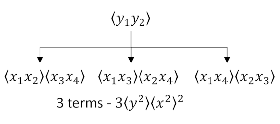
we group the $y$’s together and then form an appropriate tree of the possible combinations of $x$’s. Note that care is taken to keep the numeric labels always increasing from left to right, eliminating double counting. Once the enumeration is complete, we can remove the numeric labels and count the number of occurrences of $\langle x^2 \rangle$ with $\langle y^2 \rangle$. The answer $3 \langle x^2 \rangle^2 \langle y^2 \rangle$ matches the algebraic factor $3 B_{xx}^2 B_{yy}$.
In the second diagram
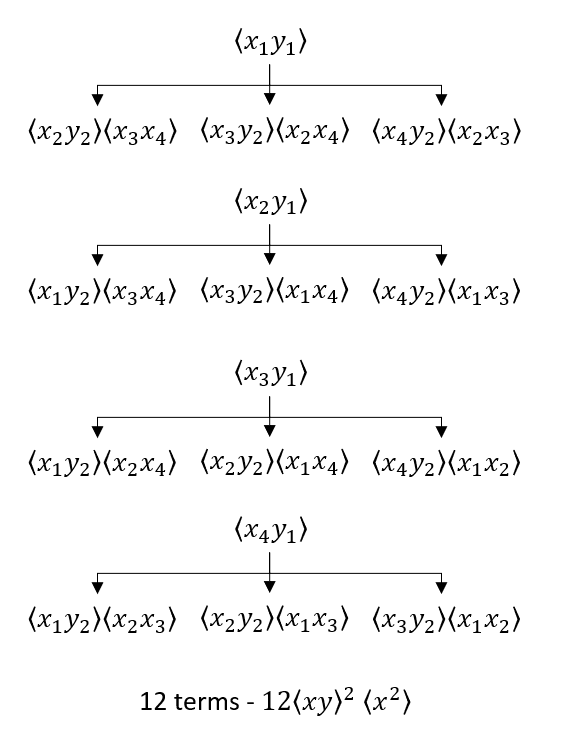
we group $y_1$ with all of the possible $x$’s (four sub-diagrams) and then proceed as above. The answer $ 12 \langle x y \rangle ^2 \langle x^2 \rangle$ matches the algebraic factor $12 B_{xx} B_{xy}^2$. It might be tempting to think that there should be an equivalent set of four sub-diagrams with $y_2$ at the top of each tree but a bit of reflection should convince us that the presence of $y_2$ in every subterm serves to arrive at the same thing without double counting. In other words, a simple reshuffling of the 12 terms can be made to have $y_2$ as the head of each sub-diagram instead of $y_1$.
As a final example, we consider a 3-dimensional case with the aim of calculating $E[x^2 y z^3]$. This expression spawns 3 diagrams:
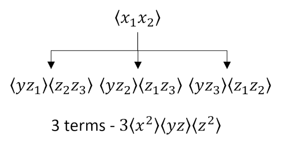
and
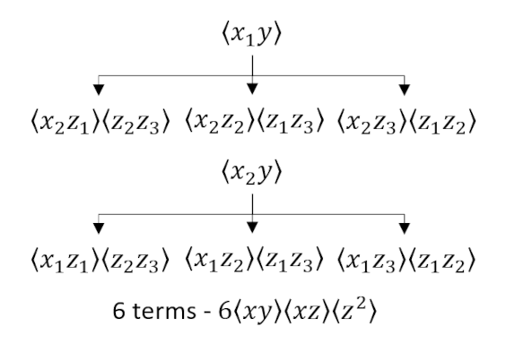
and
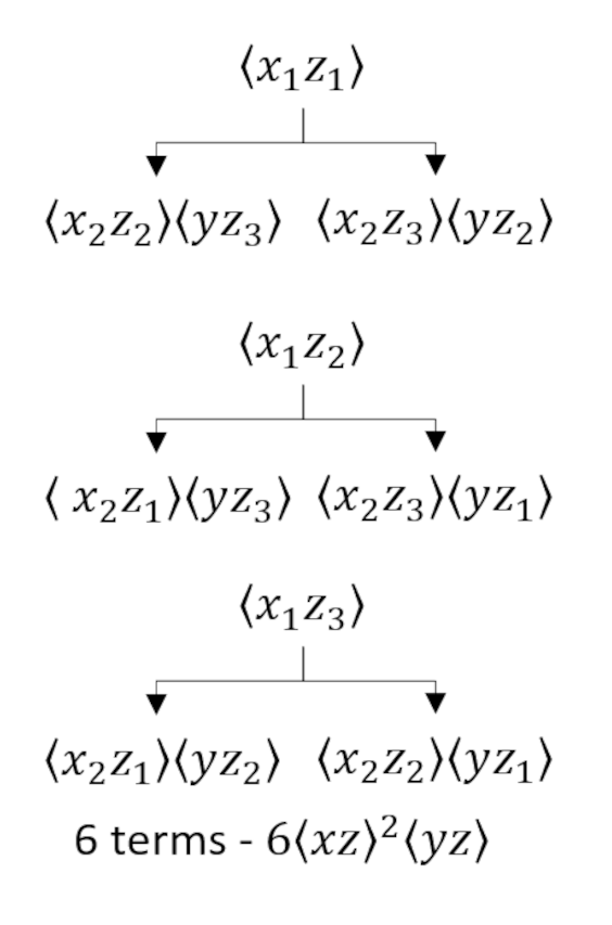
which tells us that
\[ E[x^2 y z^3] = 3 B_{xx} B_{yz} B_{zz} + 6 B_{xy} B_{xz} B_{zz} + 6 B_{xz}^2 B_{yz} \; , \]
which is confirmed by sympy computer algebra, which gave $E[x^2yz^3]: 3*Bxx*Byz*Bzz + 6*Bxy*Bxz*Bzz + 6*Bxz**2*Byz$.