
A Symbolic Experiment – Part 5: Finding Subexpressions
In the last post, we looked at how to determine if any two SymPy expressions (call them expr1 and expr2) were structurally the same and/or mathematically equivalent using the ‘==’ operator to determine structural equivalency or using ‘simplify(expr1-expr2)’ to determine mathematical equivalency. (Note that there is a built-in .equals function belonging to the expression class that performs the same function as the subtraction idiom so that ‘expr1.equal(expr2)’ yields the same results as ‘simplify(expr1-expr2)’.
However, it is often the case where we want to know if a subexpression matches some part of a larger expression’s tree as a prelude to simplification or modification of the original expression. We will confine this installment to those design patterns that combine built-in SymPy functions with relatively simple python code and will save more involved techniques that walk the expression tree for a future post.
Some of the material presented here will necessarily overlap with the concepts from the previous post since the techniques used for determining if a sub-expression is contained within a larger tree require being able to determine if the structure of a branch of larger tree matches the structure of the expression being sought.
We’ll start with the somewhat contrived but nonetheless valid mathematical expression
\[ a + \frac{1}{2} b \sin(x^2) + \frac{3}{4} c \sin^2 (x^2) + d \sin^4 (x^2) + e \sin^7 (y^2) + \frac{1}{a + \frac{x}{c}} \; . \]
with a corresponding tree that looks like
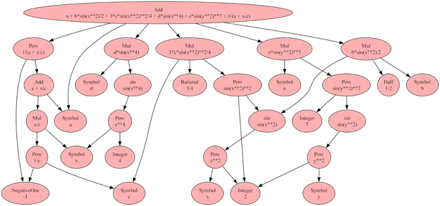
Before moving to the next step of finding sub-expressions within the original expression, a couple notes are important to set context.
First and foremost, since this example (as well as the vast majority of the examples used in SymPy documentation) is ‘known’ from the outset, it is easy to lose sight of the fact that, in general, we won’t know much (if anything) about the expression we are working with. To be concrete, here we know by initial construction and subsequent inspection that the expression, being made of the sum of 6 terms, must have an Add at the top of the expression tree. But the process of general term rewriting that is usually done in computer algebra will typically put us in a position where we will not. An excellent example of the emergence of an ‘unknown’ addition would be the case of the product rule from calculus that transforms a top node from being a product (a Mul in SymPy terms) into a sum (an Add):
\[ \frac{d}{dx} \left( f(x)g(x) \right) = f’(x)g(x) + f(x)g’(x) \; . \]
Similar issues show up in integration, where an unknown constant of integration emerges. Therefore, it is important to be able to examine a tree without any a priori knowledge about its structure.
Second, the things that we are looking for within the tree are of mixed type: some items are Atoms (Symbols, Integers, Floats, Rationals, etc.); some are Functions with the additional subdivisions into:
- base functions like Add and Mul, which exist as abstract class for most situations but which come into play when testing for addition or multiplication withing the expression;
- mathematical functions like sin, cos, or exp, which exist mostly as actual mathematical functions (e.g., sin(x)) but also show up as abstract classes when testing for their presence (e.g., Fourier expansions where we might want to test if there are no sines present due to symmetry of the expression being expanded);
- and user-defined functions like $f(x)$ and $g(x)$ where an asserted relationship exists but where no details of that relationship are either given or known a priori (e.g., solving a differential equation for a desired function).
In addition, SymPy provides some mechanisms to perform generic matching for symbols using its Wild class (e.g. sin(a+b) matches both sin(x+2) and sin(7-y), etc.).
In an operational sense, atoms form the bottom of each branch of the tree and functions are everything else that can have children. As a result of this elastic nature of functions, some additional considerations come into play when programming to find them.
With those thoughts in mind, let’s return to the original expression above. The most useful built-in functions for examining an expression tree in the programming sense (not visual inspection using graphviz) are:
- .atoms() – iterator that gives returns all the unique Atoms
- .has() – predicate Boolean that returns True if the sub-expression is found in the expression tree or False if it isn’t
- .find() – returns, in a set, all the unique instances of the sub-expression; particularly useful when trying to find a given function (e.g., sin) with a variety of different arguments.
In addition, the .args function exists that returns all the branches of the tree, but since that one is most useful in the case where we are walking the expression tree, discussion of it will be deferred to a latter post.
What follows will illustrate the basic functionality of these three functions on the original expression above, which will be designated c1. Code snippets and the results will be presented with a brief commentary afterwards.
.atoms()
Invoking .atoms():
for atom in c1.atoms():
    print(atom,'\t',type(atom))
x         <class 'sympy.core.symbol.Symbol'>
2         <class 'sympy.core.numbers.Integer'>
c         <class 'sympy.core.symbol.Symbol'>
4         <class 'sympy.core.numbers.Integer'>
b         <class 'sympy.core.symbol.Symbol'>
7         <class 'sympy.core.numbers.Integer'>
1/2       <class 'sympy.core.numbers.Half'>
d         <class 'sympy.core.symbol.Symbol'>
y         <class 'sympy.core.symbol.Symbol'>
-1        <class 'sympy.core.numbers.NegativeOne'>
e         <class 'sympy.core.symbol.Symbol'>
3/4       <class 'sympy.core.numbers.Rational'>
a         <class 'sympy.core.symbol.Symbol'>
In this output, we can see some of the variety of Atoms that SymPy provides. In addition, to Symbol, Integer, and Rational, SymPy reserves ‘special’ numbers for a half and multiplication by a minus sign, for performance sake and convenience.
.has() and .find()
These two are best understood being invoked side-by-side using a list (called queries) of the patterns we are trying to find.
Invoking .has() and .find() (with the prior ‘import SymPy as sym’):
queries = [sym.Add,
           sym.Mul,
           sym.Pow,
           sym.exp,
           sym.sin,
           x,
           sym.sin(x**2),
           sym.sin(x**2)**2,
           y**2,
           sym.Rational]

for query in queries:
    if hasattr(query,'__name__'):
        print(query.__name__,' (n):\t',c1.has(query),c1.find(query))
    elif callable(getattr(query,'__repr__',None)):
        print(query.__repr__(),' (r):\t',c1.has(query),c1.find(query))
    else:
        print(query,' ():\t',c1.has(query),c1.find(query))
Output (slightly reformatted versus the code above):
Add  (n):  True
   {a + x/c, a + b*sin(x**2)/2 + 3*c*sin(x**2)**2/4 + d*sin(x**4) + e*sin(y**2)**7 + 1/(a + x/c)}
Mul  (n):  True
   {e*sin(y**2)**7, x/c, d*sin(x**4), 3*c*sin(x**2)**2/4, b*sin(x**2)/2}
Pow  (n):  True
   {sin(x**2)**2, x**4, 1/c, 1/(a + x/c), sin(y**2)**7, y**2, x**2}
exp  (n):  False
   set()
sin  (n):  True
   {sin(x**4), sin(y**2), sin(x**2)}
x  (r):    True
   {x}
sin(x**2)  (r):  True
   {sin(x**2)}
sin(x**2)**2  (r):  True
   {sin(x**2)**2}
y**2  (r):   True
   {y**2}
Rational  (n):  True
   {2, 4, 7, 3/4, 1/2, -1}
Notice how the .find(sym.sin) returned the set {sin(x**4), sin(y**2), sin(x**2)} with all three unique instances of the sin function with different arguments not the four sin terms in c1. The powers to which some sin terms are raised are also ignored as are the coefficients multiplying them. Essentially, .find isolates in the expression tree those branches starting at sin(x**2), sin(x**4), and sin(y**2), omitting everything above. Visually, this can be represented as:
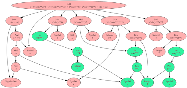
where the green ovals show what sub-trees .find has found within the larger tree.
One final note, to get the print to be as attractive as it was above (Add versus sympy.core.add.Add) one has to switch between __name__ and __repr__() as appropriate. The decoration after the string (either ‘(n)’ or ‘(r)’) signals which selection was made. This functionality is only included for debugging and understanding of the code and it doesn’t matter in any way for the actual manipulation of the trees.
Finally, it is important to see that .has() and .find() are looking for structural features and are not concerned with mathematical equivalence. To drive this point home, consider the following there ways to write the mathematically same expression:
- tree1 = mu/2/(a+b/2)
- tree2 = mu/(2*a+b)
- tree3 = mu/(2*(a+b/2))
SymPy distributes the multiplication in the denominator so that tree2 and tree3 have the exact same structure but that the double divide in tree1 leads to a different structure:
<image>
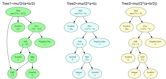
As a result, issuing tree1.has(2*a) returns a False while tree2.has(2*a) returns True (as does tree3). Likewise, tree1.has(b/2) returns True while tree2.has(b/2) returns False. In both cases, the structurally correct sub-tree is either found or not found within the larger tree.