Neural Networks 2 – The Math
coming soon

coming soon
This month’s column begins a new effort that is inspired by and strongly follows the video Building a neural network FROM SCRATCH (no Tensorflow/Pytorch, just numpy & math) by Samson Zhang. Like Zhang, I agree that the best way to learn any algorithm is to build one from scratch even if, and, more important, especially if you are going to use someone else’s code. Usually, one can’t understand the behavior nor appreciate the effort that went into an external package without having ‘walked a mile in another developer’s shoes’. You also don’t know where the algorithm is likely to work or fail if you don’t have some insight into the inner workings.
Zhang provides all of his code and data on his Kaggle notebook and that code base formed the starting point for this exploration. However, the data that were used was from the Kaggle repository by Dariel Dato-On at MNIST in CSV | Kaggle. In both cases the data are derived from the MNIST digitized and labels samples of hand-written numerical digits 0-9, some of which look like:

Each image is 28×28 pixels with values ranging from 0-255. For convenience, each image is stored in CSV format as a row consisting of 785 values. The first column contains the label for the image (i.e., ‘0’, ‘5’, ’5’, or ‘7’ for the cases above) and the remaining 784 columns the image data. The entire data set consists of 60,000 such rows. For this first experiment, 59,000 were used as training data and 1,000 as test data to evaluate the success of the net in converging into some useful state.
The basic idea of a neural network is the nonlinear transformation of input arrays to output arrays that provides a high probability of classifying the input data into the correct ‘bucket’. In this example, the input arrays are 784-length, normalized, column vectors with real values ranging $[0,1]$ and the outputs are probabilities of belonging in one of the ten possible output buckets of $[0,1,2,3,4,5,6,7,8,9]$.
Zhang’s network consists of 3-layers: an input layer consisting of 784 slots to accommodate the 784 pixels in each image; a hidden layer consisting of 10 slots, each receiving input from each slot in the previous layer (i.e., input layer), the precise mechanics of which will be discussed below; and finally an output layer consisting of 10 slots, each, again, receiving input from each slot in the previous layer (i.e., the hidden layer). Properly normalized, the values in the output layer can be interpreted as probabilities with the maximum value corresponding to the most likely label.
To be concrete, below is a schematic of how the final trained network decided that a ‘0’ input image should be classified as a ‘0’:
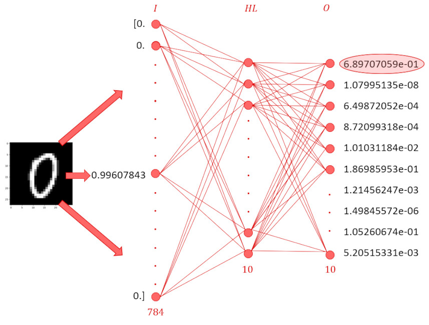
The image of the hand-written ‘0’ was converted to a one-dimensional array with 784 components, four of which are shown being fed into the input layer. Pre-determined weights and biases, $W$ and $b$ at both layers (of different sizes, of course) create an affine transformation of the results of the previous layer
\[ Z^{(1)} = W^{(1)} \cdot X^{(0)} + b^{(1)} \; , \]
where the ‘dot product’ between the $W$ and the $X$ stands for the appropriate matrix product (i.e., $W_{ij} X_{j}$). This transformation is then applied to each image in the training set (Zhang used 39,000 images; the one detailed here used 59,000 – with both cases holding back 1000 images for testing). Typically, for data sets this small, the images are stacked in a single array and fed in all at once since the average cost over the whole set is easily computed with little storage overhead. Thus, there is actually a suppressed index in Zhang’s code. This architecture will be revisited in a latter blog for data sets too large to hold completely in memory but for now Zhang’s approach is followed as closely as possible.
The input, $X^{1}$, for the next layer results from passing these $Z^{(1)}$ outputs through a nonlinear transformation before being passed onto the next layer. The nonlinearity represents the ‘activation’ of each neuron and the current best practice involves using the ReLU function defined as
\[ ReLU(x) = \left\{ \begin{array}{lc} x & x > 0 \\ 0 & {\mathrm otherwise} \end{array} \right. \; , \]
meaning that
\[ X^{(1)} = ReLU(Z^{(1)}) \; . \]
The dimensionality of each column of $Z^{(1)}$ is now 10, although different numbers of neurons in the hidden layer are also possible. This is another point deferred to a later blog.
The transformation from the hidden layer to the output layer works in much the same way with
\[ Z^{(2)} = W^{(2)} \cdot X^{(1)} + b^{(2)} \; , \]
but the nonlinear transformation to the output layer is, in this case, the SoftMax transformation that normalizes the each of the nodes on the output layer against the whole set using
\[ X^{(2)} = \frac{\exp(Z^{(2)})}{\sum \exp(Z^{(2)})} \; , \]
resulting in a functional form reminiscent, up to the sign of the exponent, of the partition function from statistical mechanics.
Of course, the classification ability of the neural network will be poor for a set of arbitrary weights and biases. The key element in training the net is to find a combination of these values that maximizes the performance of the net across the statistically available input – in other words, an optimization problem.
In the lingo of neural nets, this optimization problem is solved via the back-propagation process, which basically depends on the differentiability of the transformations and the implicit (or inverse) function theorems to determine the proper inputs given the desired outputs. The starting point is the formation of the ‘residuals’ $R$ (a term used locally here) defined as
\[ R = X^{(2)} – Y \; , \]
where $Y$ is the true or correct value for the labeled image. For the ‘0’ example above, $Y$ will look like the 10-element array
\[ Y = \left[ 1, 0, 0, 0, 0, 0, 0, 0, 0, 0 \right] \; .\]
If the label had been ‘4’, then the 1 would have been put in the corresponding spot for four, which is the fifth array element in from the left.
The equations Zhang cites for this back propagation:
\[ dZ^{[2]} = A^{[2]} – Y \; , \]
\[ dW^{[2]} = \frac{1}{m} dZ^{[2]} A^{[1]T} \; ,\]
\[ dB^{[2]} = \frac{1}{m} \Sigma {dZ^{[2]}} \; , \]
\[dZ^{[1]} = W^{[2]T} dZ^{[2]} .* g^{[1]\prime} (z^{[1]}) \; ,\]
\[ dW^{[1]} = \frac{1}{m} dZ^{[1]} A^{[0]T} \; ,\]
and
\[ dB^{[1]} = \frac{1}{m} \Sigma {dZ^{[1]}} \; .\]
These equations clearly show the backwards chaining of derivatives via the chain rule but are quite difficult to decode as he mixes notation (for example his $A$’s are also $X$’s) and intermixes some of the broadcasting rules he uses when employing numpy (hence the factor of $m$, which is the size of the number of rows in the training data set and the presence of the transposed $T$ notation) with those representing the connecting edges of the net. Nonetheless, his code for the net works reasonably well with an achieved accuracy of about 85% to 89% on the test set and it forms an excellent starting point for building a neural network from the ground up.
Next month’s blog will focus on coding the nuts and bolts of a similar network from scratch with along with a proper derivation of the back propagation.
Last month’s post established how to compute arbitrary multivariate moments of a Gaussian distribution by coupling the desired distribution with a ‘source’ term
\[ I = \int d^n r e^{(-r^T A r/2 + b^T r)} = e^{-b^T A^{-1} b/2} \, \frac{(2 \pi)^{(n/2)}}{\sqrt{\det{A}}} \; , \]
for an arbitrary positive definite matrix $A$ and a multivariate quadratic form $r^T A r$. The coupling term $b$ allows for the computation of the moments by taking derivatives with respect to $b$ and then setting $b=0$, afterwards. For example, from the last post, the multivariate moment
\[ E[x^4y^2] = \left. \frac{\partial^6}{\partial b_x^4 \partial b_y^2 } e^{b^T B b/2} \right|_{b=0} = 3 B_{xx}^2 B_{yy} + 12 B_{xx} B_{xy}^2 \; , \]
where $B = A^{-1}$.
Of course, these derivatives are easy to evaluate with modern computer algebra systems but calculating them by hand is prohibitively expensive in many cases and a variety of techniques were developed for short-cutting much of the labor that are worth knowing in their own right. One such technique is Isserlis’ Theorem, which is a way of organizing the algebra so that the computation depends only on determining $A^{-1}$ and performing some combinatorics. It is that last activity that will be the focus of this blog post.
We will be considering a general multivariate moment of the form
\[ E[x^{n_1} y^{n_2}\cdots a^{n_4} b^{n_5} \cdots] \; .\]
The first thing to note is that the total power of the moment $n = n_1 + n_2 + \cdots$ must be even in order to have a non-zero result, otherwise there will always be a residual $b$ in the result that will become null when the requirement $b=0$ is enforced. As a result we can express the total power of the moment as $n = 2m$. Second, the only surviving term in expansion of the exponential will be the $m^{\textrm{th}}$ term for similar reasons. The resulting moments are always taken pairwise because of the quadratic form of the exponential, as seen above. The only unknown is the numerical coefficient in front of the various terms.
Since we are interested in the unique pairings, it is useful to give each variable in the statistical moment a unique label in addition to its name. With this approach, $x^4 y^2 = x_1 x_2 x_3 x_4 y_1 y_2$. A total power $n$ corresponds to $n$ such unique terms and $n!$ possible permutation of a list of them. Since $n$ is even, there are $m = n/2$ pairs of consecutive terms in each list to form the $m$ individual pairs. Since the order of the pairs doesn’t matter, we divide by $m!$ to get the unique combinations of pairs and then again by a factor of $2$ for each pair to account for the fact that a pair is symmetric as to ordering; $x_1 x_2$ is equivalent to $x_2 x_1$. Racking all theses pieces up gives the number of terms as
\[ N = \frac{(2m)!}{m! 2^m} \; .\]
Regrouping the denominator as to associate with each term in $m!$ a value of $2$ gives
\[ N = \frac{2m (2m-1) (2m-2) \cdots }{ 2m (2m – 2) (2m – 4) \cdots} = (2m – 1) (2m – 3) \cdots \equiv (2m-1)!! \; . \]
For our test case of $E[x^4 y^2]$, $n=6$, $m = 3$ and $(2m – 1)!! = 15$. Since $15 = 3 + 12$, that checks.
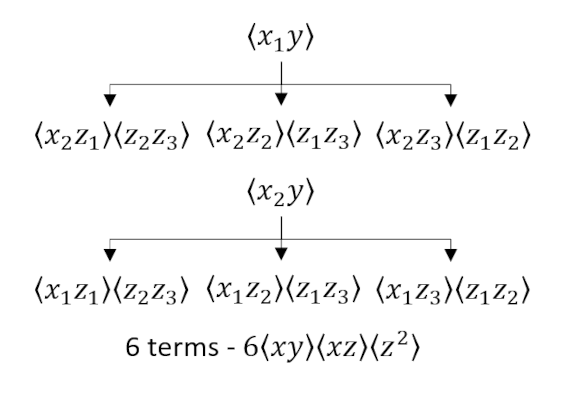
To get the specific breakdown (i.e., $15 = 3 + 12$ instead or, say, $15 = 11 + 4$) requires a bit more combinatoric work that is best explained in terms of diagrams. For convenience, we will use angle brackets instead of $E[]$ to represent expectation since the result will be easier to read, even if each term is not as expressive.
In the first diagram
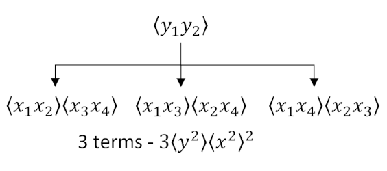
we group the $y$’s together and then form an appropriate tree of the possible combinations of $x$’s. Note that care is taken to keep the numeric labels always increasing from left to right, eliminating double counting. Once the enumeration is complete, we can remove the numeric labels and count the number of occurrences of $\langle x^2 \rangle$ with $\langle y^2 \rangle$. The answer $3 \langle x^2 \rangle^2 \langle y^2 \rangle$ matches the algebraic factor $3 B_{xx}^2 B_{yy}$.
In the second diagram
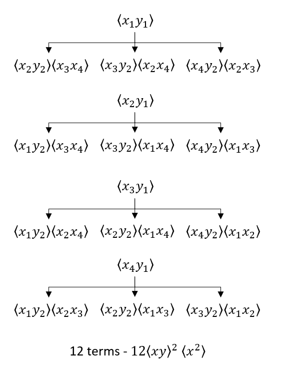
we group $y_1$ with all of the possible $x$’s (four sub-diagrams) and then proceed as above. The answer $ 12 \langle x y \rangle ^2 \langle x^2 \rangle$ matches the algebraic factor $12 B_{xx} B_{xy}^2$. It might be tempting to think that there should be an equivalent set of four sub-diagrams with $y_2$ at the top of each tree but a bit of reflection should convince us that the presence of $y_2$ in every subterm serves to arrive at the same thing without double counting. In other words, a simple reshuffling of the 12 terms can be made to have $y_2$ as the head of each sub-diagram instead of $y_1$.
As a final example, we consider a 3-dimensional case with the aim of calculating $E[x^2 y z^3]$. This expression spawns 3 diagrams:
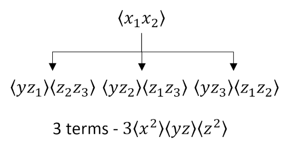
and
and
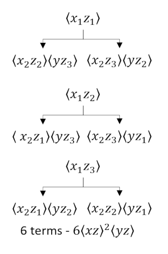
which tells us that
\[ E[x^2 y z^3] = 3 B_{xx} B_{yz} B_{zz} + 6 B_{xy} B_{xz} B_{zz} + 6 B_{xz}^2 B_{yz} \; , \]
which is confirmed by sympy computer algebra, which gave $E[x^2yz^3]: 3*Bxx*Byz*Bzz + 6*Bxy*Bxz*Bzz + 6*Bxz**2*Byz$.
This month’s blog continues the exploration begun in the last installment, which covered how to evaluate and normalize multivariate Gaussian distributions. The focus here will be on evaluating moments of these distributions. As a reminder, the prototype example is from Section 1.2 of Brezin’s text Introduction to Statistical Field Theory, where he posed the following toy problem for the reader:
\[ E[x^4 y^2] = \frac{1}{N} \int_{-\infty}^{\infty} \int_{-\infty}^{\infty} x^4 y^2 e^{-(x^2 + xy + 2 y^2)} \; , \]
where the normalization constant $N$, the value of the integral with only the exponential term kept, is found, as described in the last post, by re-expressing the exponent of the integrand as a quadratic form $r^T A r/2$ (where $r$ presents the independent variables as a column array) and then expressing the value of the integral in terms of the determinant of the matrix $A$: $N = (2 \pi)^{(n/2)}/\sqrt{\det{A}}$. Note: for reasons that will become apparent below, the scaling of the quadratic form was changed with the introduction of a one-half in the exponent. Under this scaling $A \rightarrow A/2$ and $\det{A} \rightarrow \det{A}/2^n$, where $n$ is the dimensionality of the space.
To evaluate the moments, we first extend the exponent by ‘coupling’ it to an $n$-dimensional ‘source’ $b$ via the introduction of the term $b^T r$ in the exponent. The integrand becomes:
\[ e^{-r^T A r/2 + b^T r} . \]
The strategy for manipulating this term into one we can deal with is akin to usual ‘complete the square’ approach in one dimension but generalized. We start by defining a new variable
\[ s = r \, – A^{-1} b \; .\]
Regardless of what $b$ is (real positive, real negative, complex, etc.) the original limits on the $r_i \in (-\infty,\infty)$ carry over to $s$. Likewise, the measures of the two variables are related by $d^ns =d^nr$. In terms of the integral, this definition simply moves the origin of the $s$ relative to the $r$ by an amount $A^{-1}b$, which results in no change since the range is infinite.
Let’s manipulate the first term in the exponent step-by-step. Expanding the right side gives
\[ r^T A (s + A^{-1} b) = r^T A s + r^T b \; .\]
Since $A$ is symmetric, its inverse is too, $\left( A^{-1} \right)^T = A^{-1}$ and this observation allows us to now expand the first term side, giving
\[ (s^T + b^T A^{-1} ) A s + r^T b = s^T A s + b^T s + r^T b \; . \]
Next note that $b^T r = b_i r_i = r^T b$ (summation implied) and then substitute these pieces into the original expression to get
\[ -r^T A r/2 – b^T r = -( s^T A s + b^T s + b^T r)/2 + b^T r \\ = -s^T A s + b^T ( r – s )/2 \; . \]
Finally, using the definition of $s$ the last term can be simplified to eliminate both $r$ and $s$, leaving
\[ -r^T A r = -s^T A s + b^T A^{-1} b /2 \; .\]
The original integral $I = \int d^n r \exp{(-r^T A r/2 + b^T r)}$ now becomes
\[ I = e^{-b^T A^{-1} b/2} \int d^n s \, e^{-s^T A s} = e^{-b^T A^{-1} b/2} \, \frac{(2 \pi)^{(n/2)}}{\sqrt{\det{A}}} \; . \]
This result provides us with the mechanism to evaluate any multivariate moment of the distribution by differentiating with respect to $b$ and then setting $b=0$ afterwards.
For instance, if $r^T = [x,y]$, then the moment of $x$ with respect to the original distribution of the Brezin problem is
\[ E[x] = \frac{1}{N} \int_{-\infty}^{\infty} \int_{-\infty}^{\infty} x e^{-(x^2 + xy + 2 y^2)} \; , \]
where $N = 2\pi/\sqrt{\det{A}}$.
Our expectation is, by symmetry, that this integral is zero. We can confirm that by noting that first that the expectation value is given by
\[ E[x;b] = \frac{\partial}{\partial b_x } \frac{1}{N} \int dx \, dy \, e^{-r^T A r + b_x x + b_y y} \\ = \frac{1}{N} \int dx \, dy \, x e^{-r^T A r + b_x x + b_y y} \; ,\]
where the notation $E[x;b]$ is adopted to remind us that we have yet to set $b=0$.
Substituting the result from above gives
\[ E[x] = \left. \left( \frac{\partial}{\partial b_x } e^{b^T A^{-1} b/2} \right) \right|_{b=0} \\ = \left. \frac{\partial}{\partial b_x} (b^T A^{-1} b)/2 \right|_{b=0} \; , \]
where, in the last step, we used $\left. e^{b^T A^{-1} b} \right|_{b=0} = 1$.
At this point it is easier to switch to index notation when evaluating the derivative to get
\[ E[x] = \left. \frac{\partial}{\partial b_x} (b_i (A^{-1})_{ij} b_j/2) \right|_{b=0} = \left. (A^{-1})_{xj} b_j \right|_{b=0} = 0 \; ,\]
where rationale for the scaling by $1/2$ now becomes obvious.
At this point, we are ready to tackle the original problem. For now, we will use a symbolic algebra system to calculate the required derivatives, deferring until the next post some of the techniques needed to simplify and generalize these steps. In addition, for notational simplicity, we assign $B = A^{-1}$.
Brezin’s problem requires that
\[ A = \left[ \begin{array}{cc} 2 & 1 \\ 1 & 4 \end{array} \right] \; \]
and that
\[ B = A^{-1} = \frac{1}{7} \left[ \begin{array}{cc} 4 & -1 \\ -1 & 2 \end{array} \right] \; .\]
The required moment is related to the derivatives of $b^T B b$ as
\[ E[x^4y^2] = \left. \frac{\partial^6}{\partial b_x^4 \partial b_y^2 } e^{b^T B b/2} \right|_{b=0} = 3 B_{xx}^2 B_{yy} + 12 B_{xx} B_{xy}^2 \; . \]
Substituting from above yields
\[ E[x^4 y^2] = 3 \left( \frac{4}{7} \right)^2 \frac{2}{7} + 12 \frac{4}{7} \left( \frac{-1}{7} \right)^2 \; , \]
which evaluates to
\[ E[x^4 y^2] = \frac{96}{343} + \frac{48}{343} = \frac{144}{343} \; . \]
A brute force Monte Carlo evaluation gives the estimate $E[x^4 y^2] = 0.4208196$ compared with the exact decimal representation of $0.4198251$, a $0.24\%$ error, which is in excellent agreement.
In this month’s blog, we explore some of the statistical results from multivariate Gaussian distributions. Typically, many of these results were developed in support of particular problems in science and engineering, but they stand on their own in that the results flow from the logic of statistical thinking that can be cleanly separated from the application that birthed them.
The Monte Carlo method, which was the subject in a previous run of blogs (Monte Carlo Integration, Part 1 to Part 5), will be used here as an additional check on the techniques developed, but there will be no emphasis on the mechanics of these techniques.
For a typical, motivating example, consider the expectation value presented in Section 1.2 of Brezin’s text Introduction to Statistical Field Theory, which asks the reader to compute
\[ E[x^4 y^2] = \frac{1}{N} \int_{-\infty}^{\infty} \int_{-\infty}^{\infty} x^4 y^2 e^{-(x^2 + xy + 2 y^2)} \; , \]
where the normalization constant $N$ is given by
\[ N = \int_{-\infty}^{\infty} \int_{-\infty}^{\infty} e^{-(x^2 + xy + 2 y^2)} \; . \]
Examples like these arise in any discipline where the model describing a system depends on several (perhaps a huge number of) parameters that manifest themselves as inter-correlated variables that we can measure. The cross-correlation between the variables $x$ and $y$ is displayed by the $xy$ term in the exponential.
The first task in determining the expectation value is to evaluate the normalization constant. The general method for solving this task will be the focus of this installment.
The method for integrating Gaussian integrals in one dimension is well known (see, e.g., here) but the approach for multivariate distributions is not as common. The first point is to look at the quadratic form in the argument of the exponential as being built as the inner product between an array presenting the variables $x$ and $y$ and some matrix $A$. In the present case this is done by recognizing
\[ x^2 + xy + 2 y^2 = \left[ \begin{array}{cc} x & y \end{array} \right] \left[ \begin{array}{cc} 1 & 1/2 \\ 1/2 & 2 \end{array} \right] \left[ \begin{array}{c} x \\ y \end{array} \right] \; . \]
Looking ahead to higher dimensional cases, we can see that this expression can be written more generally and compactly as $r^T A r \equiv r_i A_{ij} r_j$, where $r$ is a column array presenting the independent variable of the distribution (now imagined to be $n$ in number) and $A$ is a real $n \times n$ matrix; the superscript $T$ indicates that the transpose of the original array is being used.
With this new notation, any $n$-dimensional Gaussian distribution can now be written as
\[ e^{-(r^T A r)} \; . \]
Since this expression is symmetric in $r$, $A$ can be taken to be symmetric without loss of generality. This observation guarantees that $A$ can be diagonalized by an orthogonal matrix $M$ such that $M^T A M = D$, $M^T M = M M^T = 1$, and $D$ is a diagonal matrix. This, in turn, means that the quadratic form can be rewritten as
\[ r^T A r = r^T (M M^T) A (M M^T) r = \\ (r^T M) (M^T A M) (M r) = (r^T M) D (M^T r) \; . \]
The next step is to define a new set of variables defined by $s = M^T r$, which then decouples the multivariate distribution into a product of $D$ independent one-dimensional Gaussians:
\[ e^{ – (r^T A r) } = e^{ – (s^T D s) } = \prod_{i=1}^{n} e^{-d_i s_i^2} \; , \]
where the $\{d_i\}$ are the individual, on-diagonal elements of $D$ and the $\{s_i\}$. For the integral to exist (i.e., converge), we need one additional stipulation: that all of the $d_i > 0$. Said differently, we require that $A$ have positive eigenvalues (i.e., be positive definite).
The final step is to recognize that the measure of the integral changes in a convenient way when we make the substitution $r = M^T s$, since
\[ d^n r = det(M^T) d^n s = d^n s \; , \]
where we’ve exploited the fact that, since $M$ is orthogonal, its determinant is 1.
Putting all of these pieces together we now have
\[ \int_{R^n} d^n e^{-(r^T A r} = \int_{R^n} d^n s \prod_{i=1}^n e^{-d_i s_i^2} = \prod_{i=1}^{n} \int_{-\infty}^\infty ds_i e^{-d_i s_i^2} \; .\]
Since the right-hand side is a product of independent Gaussian integrals, it simplifies to
\[\prod_{i=1}^{n} \int_{-\infty}^\infty ds_i e^{-d_i s_i^2} = \prod_{i=1}^{n} \sqrt{\frac{\pi}{d_i}} = \frac{\pi^{n/2}}{\sqrt{d_1 \cdots d_n}} \; . \]
The denominator of the last expression is the determinant of the $D$, which is also the determinant of $A$. So, the final formula is
\[ \int_{R^n} d^n r e^{-(r^T A r)} = \frac{\pi^{n/2}}{\sqrt{det(A)}} \; .\]
Returning to the original example, the formula tells us that, since $det(A) = 7/4$, then the normalization constant $N = 2\pi/\sqrt(7) \approx 2.37482$. We can confirm this using brute force Monte Carlo by uniformly sampling across the ranges $x \in [-6,6]$ and $y \in [-12,12]$. The limits of these ranges were selected by going out roughly to 6 times the respective eigenvalue ($d_x = 0.79$, $d_y = 2.21$), but the estimated integral is insensitive to fine details as long as the computational domain is sufficiently large. That said, there is an art to picking the computational domain, and sophisticated pieces of software are designed to adjust to the integrand. Implementing the brute force Monte Carlo in python gave an estimate of $N = 2.37661$ for 10 million trials, an error of less than $0.1\%$.
As a last sample, suppose we provide a bigger matrix given by:
\[ A = \left[ \begin{array}{cccc} 3 & 1 & 5 & 3\\ 1 & 5 & 2 & 0\\ 5 & 2 & 10 & 3 \\ 3 & 0 & 3 & 14 \end{array} \right] \; .\]
The Gaussian integral is
\[ N = \int_{R^n} d^n r \, e^{-(3w^2 + 2wx + 10wy + 6w^2 + 5x^2 + 4xy + 10y^2 + 6yz + 14z^2)} \; .\]
The eigenvalues of $A$ are: $\{17.63,0.26,9.85,4.26\}$. Application of the formula gives $N = 0.70497$ compared with a brute force Monte Carlo estimate of $0.71061$.
With this operation well in hand, next month’s post will focus on calculating various moments of these distributions.
One of the persistent mysteries surrounding that art form that is called the mystery is exactly how to write a good one. Of course, there’s no denying that a command of the English language is essential. So too is the ability to create such engaging characters that we want don’t want the mystery to end. Indeed, the masters, such as Arthur Conan Doyle, G.K. Chesterton, Rex Stout, and Agatha Christie created such enduring characters that we enjoy visiting them again and again regardless of the crime underfoot. And having a victim, either totally sympathetic or entirely loathsome, is important so that we can either enjoy righteous justice being meted out or secretly delight in someone getting what’s coming to him. But foremost is the requirement, agreed to by tacit contract by the writer with the reader, that the detective’s solution be a satisfying explanation with surprises and ‘aha’ moments that nonetheless ties up all the loose ends. As Chesterton puts it, the writer should provide a simple explanation of something that only appears complex; an explanation that doesn’t, itself, need an explanation.
There are several, classic ways that authors employ to add complexity to a mystery, to obscure what’s going on. These include the red herring, in which an event or a set of clues lead nowhere and only serve as dust to cover the real trail. Another classic approach is to provide so many extraneous details, typically by indulging in sumptuous descriptions of surroundings or detailed appearance and behaviors of the characters, that a vital clue is lost amid noise. And, of course, there are accusations of authors who withhold vital clues and omit important details as is hilariously summarized in the final act of the movie Murder by Death.
Omitting vital clues or important information is commonly considered unfair; a bad show which is against the rules of the implicit contract discussed above. And yet, there is a way to omit something from a mystery while still playing fair with the reader. This fair-play omission occurs when the writer leaves out the second of the Three Acts of the Mind thereby leaving out a judgement or predication of the facts already revealed, which any reader with common sense can make for himself but usually doesn’t.
For those unfamiliar with what philosophers mean by the three acts of the mind, a terse summary must suffice. The first act of the mind shows that mental faculty that allows a thing to grasp what is being observed. For example, it is the ability we all possess to look a room and distinguish a chair from the pistol resting on the seat. In the second act of the mind, a predication about some object observed in the first act is made such as the pistol is smoking. The third act of the mind ties the various observations and their corresponding predications together with connective reasoning to conclude something like: since the pistol is still smoking and the cause of death is a bullet wound, the murder must have committed the crime only a short time before.
Omitting the second act of the mind doesn’t violate the contract since it neither steals a simple clue from the reader’s notice nor does it hide a clue in plain sight by requiring the reader to have narrow, specialized knowledge to understand it. Rather, the writer shares information freely but doesn’t spoon feed the proper interpretation, relying, instead on the reader to provide it for himself.
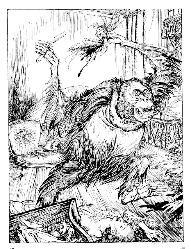
An excellent example of how to omit the second act of the mind and thereby write an engaging mystery is Edgar Allen Poe’s Murders in the Rue Morgue.
This mystery, told by an unnamed narrator, centers on the horrific deaths of Madame L’Espanaye and her daughter Mademoiselle Camille L’Espanaye. Both victims were “frightfully mutilated” with the mother being essentially decapitated by murderer using nothing more than an ordinary straight razor while the daughter’s battered and strangled corpse was shoved, head-down, up the chimney so far that the body “could not be got down until four or five of the party united their strength.”
Poe makes the mystery even more interesting by proving scores of witnesses who heard the screams of the women as the crime was unfolding. A subset of these followed a gendarme into the house after the latter had forced entry and arrived on the scene, an upper-floor bedroom, in time to find the daughter’s corpse still warm. The door from the hall into the bedroom was locked from the inside, the room itself was in shambles with the furnishings thrown about, and all its window were closed and locked. Each of the witnesses who ascended the house during the murder testified to hearing two voices coming from above in “angry contention.” The first voice was universally agreed to be the gruff voice of a French-speaking male. The second voice, variously described as shrill or harsh, defied classification of the witnesses. A French man thought the voice to be speaking Italian; an English man thought it to be German; a Spaniard thought it English; and so on.
Having laid out the facts, Poe then allows the reader some space before having his detective, C. Auguste Dupin, fill in the gaps. Dupin provides the judgement (i.e., predication) of the facts that serve as the connective tissue between the simple apprehension of the facts (e.g., two voices in angry contention) and the solution of the crime.
Several of the interpretations that Dupin provides us become clear after their revelation but none so arresting as his insight into the inability of none witness to agree on the nationality of the shrill or harsh voice. Poe puts in marvelously in this exchange between the Dupin and the narrator:
Let me now advert – not to the whole testimony respecting these voices – but to what was peculiar in that testimony. Did you observe any thing peculiar about it?”
I remarked that, while all the witnesses agreed in supposing the gruff voice to be that of a Frenchman, there was much disagreement in regard to the shrill, or, as one individual termed it, the harsh voice.
“That was the evidence itself,” said Dupin, “but it was not the peculiarity of the evidence. You have observed nothing distinctive. Yet there was something to be observed. The witnesses, as you remark, agreed about the gruff voice; they were here unanimous. But in regard to the shrill voice, the peculiarity is – not that they disagreed – but that, while an Italian, an Englishman, a Spaniard, a Hollander, and a Frenchman attempted to describe it, each one spoke of it as that of a foreigner.
From this “peculiarity” in the testimony, Dupin supports the conclusion, arrived at deductively through the exercise of the third act of the mind, that the murderer was an orangutan.
This technique is not limited to Poe alone. Consider the notable example found in Some Buried Caesar by Rex Stout. The reader is given all the necessary facts about a bull accused on goring a man to death. Indeed, the reader is just about spoon fed them just after the murder in a manner as plain as they would be presented in the final explanation. Nonetheless, the solution remains surprising for many of us precisely because we don’t provide the correct predication.
While it is likely that host of authors use this technique, whether knowingly or instinctively, it is curious that the explicit connection what makes a satisfying solution to a mystery and the omission of the second act of the mind to ‘hide’ the solution in plain sight seems never to have been made. And that is an omission we hope to correct.
As discussed in other posts, humor is a delicate thing even for rational (at least sometimes) human beings let alone for a machine intelligence the grasp. Case in point, a little joke that sneakily crept up on me all I was in a pub on a beach holiday. It was the kind of joke that at first you likely don’t get and then the light bulb goes on after a few seconds and then the subtly of the humor hits you, much like that ‘ah-ha’ moment when you finally got the Pythagorean theorem or riding a bike or some other experiential thing.
The name of the place is Shenanigans.

Given that it is an Irish Pub, it’s hardly a surprise that the dining area would stimulate its public with various pieces of trivia and witticisms. Some of these witticisms extended beyond the usual humorous ones one would expect in a conventional bar setting and bordered on wisdom. One in particular opened vistas of thought about language, meaning, ambiguity, and humor.The witticism in question, which really caught my attention, asked the following question:
Why does a dish towel get wet when it dries?
The obvious answer, of course, depends on an equivocation in the verb to dry.In English, the action of drying can be interpreted as two distinct and opposite sequence of events. In the first, we have the passion – that is to say, the passive event – of an object as it dries out. In this case, the object loses any water or other such liquid that it has been carrying or holding. An excellent example of this being the ground drying after the sun has come out after a rainfall. The object is simply bystander as it is subjected to the drying action performed by an external entity. In the second, we have the action – that is to say, the active performance – of the entity that performs the drying action. In the wet ground example mentioned earlier, the sun would perform the drying. In older language that, sadly, has fallen out of favor, the sun is the drier and the ground the ‘driee’.
Getting back to the witticism, the humor, obviously turns on the fact that the verb ‘dry’ is ambiguous in the present tense. Consider the two sentences:
The towel dries in the sun.
and
The towel dries the dish.
The first three words of each are identical with the same subject and verb. The only clue that the first is the passive sense and the second the active one is the inclusion of the prepositional phrase ‘in the sun’.
At first glance, one might think that indicator is sufficient and a bit of parsing here and a bit of coding with a lookup table there and one has taught a machine to tell the difference. Then one nips out to the pint and while drinking a pint of Guinness one realizes that the next sentence can be said with proper meaning and with equal probability of being either passive or active.
The towel dries fast.
What’s a machine to do, you may ask? Well… if it is to pass the Turing test it might randomly make an assumption and move forward or ask for clarification. If the machine were being really ‘clever’ it might do both.
Our journey through various Monte Carlo techniques has been rich and rewarding but has been confined almost exclusively to one-dimensional sampling. Even the case of the sunny/rainy-day multi-state Markov Chain (prelude and main act) was merely a precursor to the setup and analysis of the Metropolis-Hastings algorithm that was then applied in one dimension. This month, we step off the real number line and explore the plane to understand a bit of how multivariate sampling works and the meaning of covariance.
To start, let’s imagine that we are measuring the height and weight of some mythical animal, say the xandu of C.S. Friedman’s Coldfire Trilogy. Further suppose that we’ve measured 5000 members of the population and recorded their height and weight. The following figure shows the distribution of these two attributes plus the quantitative statistics of the mean and standard deviation of each.
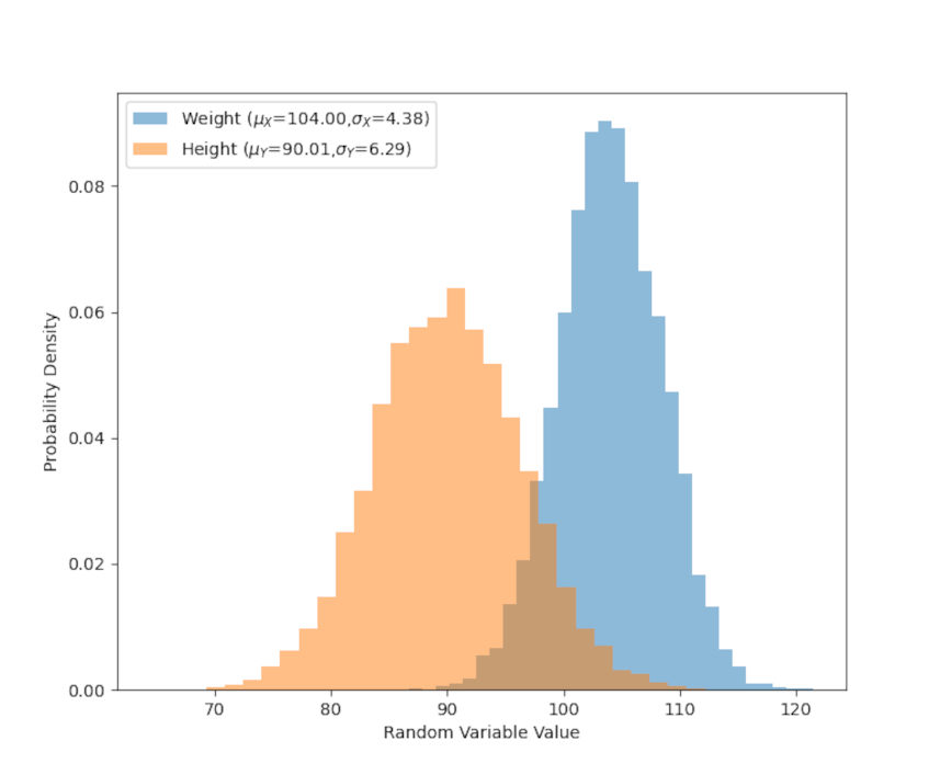
While these statistics give us a good description of the distribution of the weight or the height of the xandu population that don’t say anything about the connection between these two attributes. Generally, we would expect that the larger an animal is the heavier that animal will be, all others things being equal. To better understand the relationship between these two population characteristics, we first make a scatter plot of their weight arbitrarily displayed on the x-axis ($X$ will hereafter be a stand in symbol for weight) and their height along the y-axis ($Y$ for height).
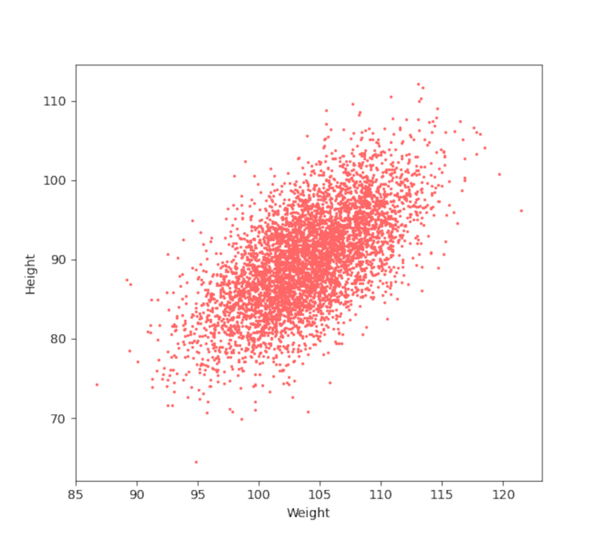
It is obvious that the two attributes are strongly correlated. To make that observation quantitative we first define the covariance matrix between the two series. Let’s remind ourselves that the variance of a set of $N$ values of the random variable $X$, denoted by ${\mathbf X} = \left\{ x_1, x_2, \ldots , x_N\right\}$ defined as
\[ {\sigma_X}^2 = \frac{1}{N} \sum_{i=1}^N \left( x_i – {\bar x} \right)^2 \; , \]
where ${\bar x}$ is the mean value given by
\[ {\bar x} = \frac{1}{N} \sum_{i=1}^N x_i \; . \]
We can express these relations more compactly by defining the common notation of an expectation value of $Q$ as
\[ E[Q] = \frac{1}{N} \sum_{i=1}^N q_i \; , \]
where $Q$ is some arbitrary set of $N$ values denoted as $q_i$. With this definition, the variance becomes
\[ {\sigma_X}^2 = E \left[ (X – {\bar x})^2 \right] \; . \]
The covariance is then the amount the set $X$ moves with (or covaries) with the set $Y$ defined by
\[ Cov(X,Y) = E \left[ (X – {\bar x}) (Y – {\bar y} ) \right] \; .\]
Note that the usual variance is now expressed as
\[ {\sigma_X}^2 = Cov(X,X) = E \left[ (X – {\bar x}) (X – {\bar x}) \right] = E \left[ (X – {\bar x})^2 \right] \; , \]
which is the same as before.
There are four unique combinations: $Cov(X,X)$, $Cov(X,Y)$, $Cov(Y,X)$, and $Cov(Y,Y)$. Because the covariance in symmetric in its arguments $Cov(Y,X) = Cov(X,Y)$. For reasons that will become clearer below, it is convenient to display these four values in the covariance matrix
\[ {\mathcal P}_{XY} = \left[ \begin{array}{cc} Cov(X,X) & Cov(X,Y) \\ Cov(Y,X) & Cov(Y,Y) \end{array} \right] \; , \]
where it is understood that in real computations the off-diagonal terms are symmetric.
The computation of the covariance matrix for the data above is
\[ {\mathcal P}_{XY} = \left[ \begin{array}{cc} 19.22857412 & 17.51559386 \\ 17.51559386 & 39.54157185 \end{array} \right ] \; . \]
The large off-diagonal components, relative to the size of the on-diagonal components, reflects the strong correlation between weight and height of the xandu. The actual correlation coefficient is available from the correlation ${\bar {\mathcal P}}_{XY}$ matrix defined as dividing the terms by the standard deviation of the arguments used
\[ {\bar {\mathcal P}}_{XY} = \left[ \begin{array}{cc} Cov(X,X)/{\sigma_X}^2 & Cov(X,Y)/\sigma_X \sigma_Y \\ Cov(Y,X)/\sigma_Y \sigma_X & Cov(Y,Y)/{\sigma_Y}^2 \end{array} \right] \; .\]
Substituting the values in yields
\[ {\bar {\mathcal P}}_{XY} = \left[ \begin{array}{cc} 1.00000 & 0.63577 \\ 0.63577 & 1.0000 \end{array} \right ] \; . \]
The value of 0.63577 shows that the weight and height are moderately correlated so that about 64% of the variation of the one explains the variation of the other.
With these results in hand, let’s return to why it is convenient to display the individual covariances in matrix form. Doing so allows us to use the power of linear algebra to find the independent variations, $A$ and $B$, of the combined data set. When the weight-height data are experimentally measured, the independent variations are found by diagonalizing the covariance matrix. The resulting eigenvectors indicate the directions of independent variation (i.e., $A$ and $B$ will be expressed as some linear combination of $X$ and $Y$) and the eigenvalues are the corresponding variances ${\sigma_A}^2$ and ${\sigma_B}^2$. The eigenvector/eigenvalue decomposition rarely yields results that are generally understandable as the units of the two variables different but, nonetheless, one can think of the resulting directions as arising from a rotation in the weight-height space.
Understanding is best achieved by using a contrived example where we start with known population parameters for $A$ and $B$ and ‘work forward’. For this example, $\mu_A = 45$ and $\mu_B = 130$ with the corresponding standard deviations of $\sigma_A = 3$ and $\sigma_B = 7$, respectively. These data are then constructed so that they differ from $X$ and $Y$ by a 30-degree rotation. In other words, the matrix equation
\[ \left[ \begin{array}{c} X \\ Y \end{array} \right] = \left[ \begin{array}{cc} \cos \theta & \sin \theta \\ -\sin \theta & \cos \theta \end{array} \right] \left[ \begin{array}{c} A \\ B \end{array} \right] \; \]
relates the variations in $A$ and $B$ to the variation in $X$ and $Y$, where $\theta = 30^{\circ}$. It also relates the mean values by
\[ \left[ \begin{array}{c} \mu_X \\ \mu_Y \end{array} \right] = \left[ \begin{array}{cc} \cos \theta & \sin \theta \\ -\sin \theta & \cos \theta \end{array} \right] \left[ \begin{array}{c} \mu_A \\ \mu_B \end{array} \right] \; , \]
yielding values of $\mu_X = 103.97114317$ and $\mu_Y = 90.08330249$. Note that these are exact values and that the means calculated earlier are estimates based on the sampling.
The exact covariance can also be determined from
\[ {\mathcal P}_{XY} = M {\mathcal P}_{AB} M^{T} \; , \]
where the diagonal matrix ${\mathcal P}_{AB} = diag({\sigma_A}^2,{\sigma_B}^2)$ reflects the fact that $A$ and $B$ are independent random variables and where the ‘$T$’ superscript means the transpose. The exact value is
\[ {\mathcal P}_{XY} = = \left[ \begin{array}{cc} 19.0 & 17.32050808 \\ 17.32050808 & 39.0 \end{array} \right] \; . \]
Again, note both the excellent agreement with what has been estimated from the sampling.
These methods generalize to arbitrary dimension straightforwardly.
Finally, all of the sampling here was done using numpy, which conveniently has a multivariate sampling method. The only draw back is that it requires knowledge of the exact means and covariances so the above method of mapping $A$ and $B$ to $X$ and $Y$ is necessary. It is instructive to see how well the multivariate sampling matches the method used above in both scatter plot
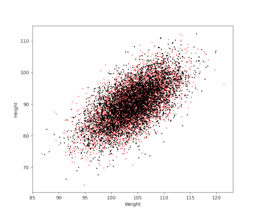
and in the individual distributions for weight
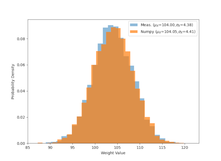
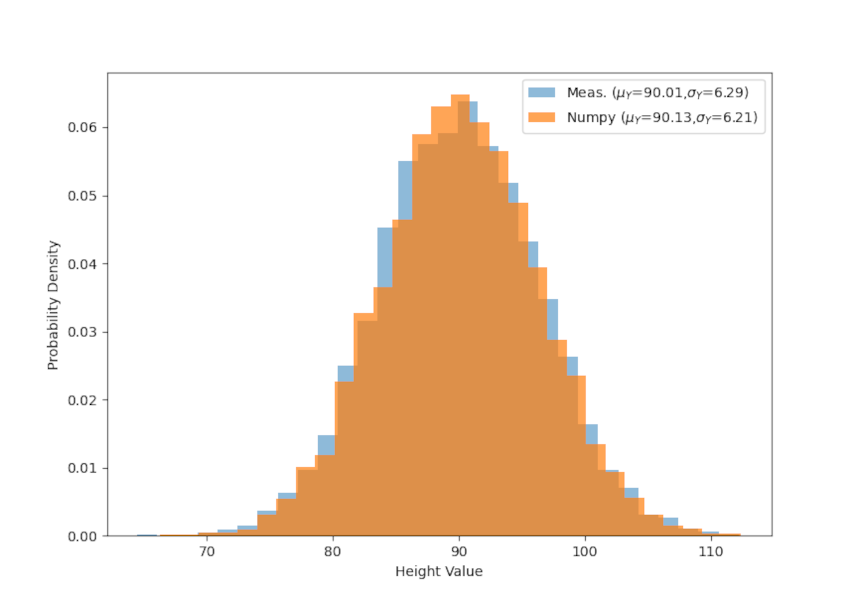
and height
Last month’s posting introduced the Metropolis-Hastings (MH) method for generating a sample distribution from just about any functional form. This method can in handy particularly for methods that are analytically intractable so that the inverse-transform method would be useless and for which the accept-reject method would be too inefficient.
The Metropolis-Hastings algorithm, which is particular instance of the broader Markov Chain Monte Carlo (MCMC) methods, brings us the desired flexibility at the expense of being computationally more involved and expensive. As a reminder, the algorithm works as follows:
and the explicit promise of this month’s installment was the explanation as to why this set of rules actually works.
Technically speaking, the algorithm, as written above, is strictly the Metropolis-Hastings algorithm for the case where the simple distribution $g(x|x_{cur})$ is symmetric; the modification for the case of non-symmetric distributions will emerge naturally in the course of justification for the rules.
The arguments presented here closely follow the excellent online presentation by ritvikmath:
To start, we relate our distribution $f(x)$ to the corresponding probability by
\[ p(x) = \frac{f(x)}{N_C} \; , \]
where $N_C$ is the normalization constant that is usually impossible to calculate analytically either because the functional form of $f(x)$ possess no analytic anti-derivative or the distribution is defined in high dimensions or both.
The MH algorithm pairs $p(x)$ with a known probability distribution $g(x)$ but in a way such that the algorithm ‘learns’ where to concentrate its effort by having $g(x)$ follow the current state around (in contrast to the accept-reject method where $g(x)$ is stationary). At each step, the transition from the current state $a$ to the proposed or candidate next state $b$ happens according to the transition probability
\[ T(a \rightarrow b) = g(b|a) A(a \rightarrow b) \; , \]
where $g(b|a)$ is conditional draw from $g(x)$ centered on state $a$ (i.e., $g$ follows the current state around) and the transition probability $A(a \rightarrow b)$ is the MH decision step. The right-hand-side of the transition probability directly maps $g(b|a)$ and $A(a \rightarrow b)$ to the first two and the last two sub-bullets of the execution step above, respectively.
To derive the MH decision step correctly describes $A(a \rightarrow b)$, we impose detailed balance,
\[ p(a) T(a \rightarrow b) = p(b) T(b \rightarrow a) \; \]
guaranteeing that the MCMC will eventually result in a stationary distribution. That detailed balance give stationary distributions of the Markov chain is most easily seen by summing both sides over $a$ to arrive at a matrix analog of the stationary requirement ${\bar S}^* = M {\bar S}^*$ used in the Sunny Day Markov chain post.
The next step involve a straightforward plugging-in of earlier relations to yield
\[ \frac{f(a)}{N_C} g(b|a) A(a \rightarrow b) = \frac{f(b)}{N_C} g(a|b) A(b \rightarrow a) \; . \]
Collecting all of the $A$’s over on one side gives
\[ \frac{A(a \rightarrow b)}{A(b \rightarrow a)} = \frac{f(b)}{f(a)} \frac{g(a|b)}{g(b|a)} \; . \]
Next define, for convenience, the two ratios
\[ R_f = \frac{f(b)}{f(a)} \; \]
and
\[ R_g = \frac{ g(a|b) }{ g(b|a) } \; . \]
Note that $R_f$ is the ratio defined earlier and that $R_g$ is exactly 1 when the $g(x)$ is a symmetric distribution.
Now, we analyze two separate cases to make sure that the transitions $A(a \rightarrow b)$ and $A(b \rightarrow a)$ can actually satisfy detailed-balance.
First, if $R_f R_g < 1$ then detailed balance will hold if we assign $A(a \rightarrow b) = R_f R_g$ and $A(b \rightarrow a) = 1$. These conditions mean that we can interpret $A(a \rightarrow b)$ as a probability for making the transition and we can then draw a number $q$ from a uniform distribution to see if we beat the odds $q \leq R_f R_g$, in which case we transition to the state $b$.
Second, if $R_f R_g \geq 1$ then detailed balance will hold is we assign $A(a \rightarrow b) = 1$ and $A(b \rightarrow a) = R_f R_g$. These conditions mean that we can interpret $A(a \rightarrow b)$ is being a demand, with 100% certainty, that we should make the change.
These two cases, which comprise the MH decision rule, are often summarized as
\[ A(a \rightarrow b) = Min(1,R_f R_g) \; \]
or, in the case when $g(x)$ is symmetric
\[ A(a \rightarrow b) = Min\left(1,\frac{f(b)}{f(a)}\right) \; , \]
which is the form used in the algorithm listing above.
The last two columns explored the notion for transition probabilities, which are conditional probabilities that express the probability of a new state being realized some system given the current state that the system finds itself in. The candidate case that was examined involved the transition probabilities of between weather conditions (sunny-to-rainy, sunny-to-sunny, etc.). That problem yielded answers via two routes: 1) stationary analysis using matrix methods and 2) Markov Chain Monte Carlo (MCMC).
The analysis of the weather problem left one large question looming. Why anyone would ever use the MCMC algorithm when the matrix method was both computationally less burdensome and also gave exact results compared to the estimated values that naturally arise in an Monte Carlo method.
There are many applications but the most straightforward one is the Metropolis-Hasting algorithm for producing pseudorandom numbers from an arbitrary distribution. In an earlier post, we presented an algorithm for producing pseudorandom numbers within a limited class of distributions using the Inverse Transform Method. While extremely economical the Inverse Transform Method depends on the finding invertible relationship between a uniformly sampled pseudorandom number $y$ and the variable $x$ that we want distributed according to some desired distribution.
The textbook example of the Inverse Transform Method is the exponential distribution. The set of pseudorandom numbers given by
\[ x = -\ln (1-y) \; , \]
where $y$ is uniformly distributed on the interval $[0,1]$, is guaranteed to be distributed exponentially.
If no such relationship can be found, the Inverse Transform Method fails to be useful.
The Metropolis-Hastings method is capable to overcoming this hurdle at the expense of being computationally much more expensive. The algorithm works as follows:
The bulk of this algorithm is very straightforward and simple. The only confusing part is the Metropolis-Hastings decision rule in the last step and why it requires the various pieces above to work. The next post will be dedicated to a detailed discussion of that rule. For now, we’ll just show the algorithm in action with various forms of $f(x)$ which are otherwise intractable.
The python code for implementing this algorithm is relatively simple. Below is a snippet from the implementation that produced the numerical results that follow. The key points to note are:
In addition to these input parameters, the value $f = N_{kept}/N_{trials}$ was reported. The rule of thumb for Metropolis-Hastings is to have a value $0.25 \leq f \leq 0.33$.
x_lim    = 2.8
N_trials = 1_000_000
delta    = 7.0
Ds       = (2*random(N_trials) - 1.0)*delta
Rs       = random(N_trials)
n_accept = 0
n_burn   = 1_000
x_0      = -2.0
x_cur    = x_0
prob     = pos_tanh
p_cur    = prob(x_cur,-x_lim,x_lim)

x = np.arange(-3,3,0.01)
z = np.array([prob(xval,-x_lim,x_lim) for xval in x])

kept = []
for d,r in zip(Ds,Rs):
    x_trial = x_cur + d
    p_trial = prob(x_trial,-x_lim,x_lim)
    w       = p_trial/p_cur
    if w >= 1 or w > r:
        x_cur = x_trial
        n_accept += 1
        if n_accept > n_burn:
            kept.append(x_cur)
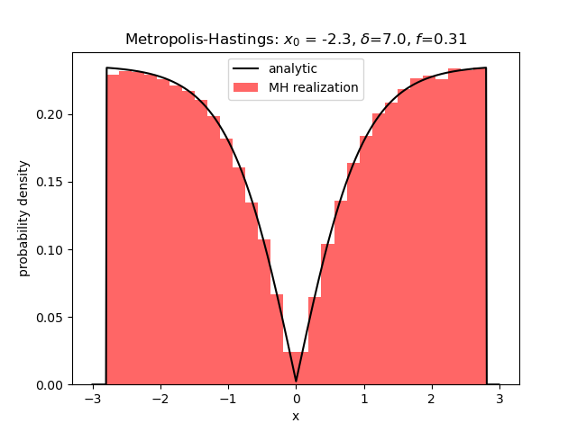
Two arbitrary and difficult functions were used for testing the algorithm: $f_1(x) = |tanh(x)|/N_1$ and $f_2(x) = \cos^6 (x)/N_2$. $N_1$ and $N_2$ are normalization constants obtained by numerically integrating over the range $[-2.8,2.8]$, which was chosen for strictly aesthetic reasons (i.e., the resulting plots looked nice).
The two parameters that had the most impact of the performance of the algorithm were the values of delta and x_0. The metric chosen for the ‘goodness’ of the algorithm is simply a visual inspection of how well the resulting distributions matched the normalized probability density functions $f_1(x)$ and $f_2(x)$.
This distribution was chosen since it has a sharp cusp in the center and two fairly flat and broad wings. The best results came from a starting point $x_0 = -2.3$ over in the left wing (the right wing also worked equally well) and a fairly large value of $\delta=7.0$ was chosen such that $f \approx 1/3$. The agreement is quite good.
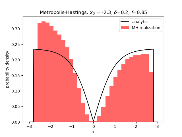
A smaller value of $\delta$ lead to more samples being collected ($f=0.85$) but the realizations couldn’t ‘shake off the memory’ that they started over in the left wing and the results were not very good, although the two-wing structure can still be seen.
Starting off with $x_0 = 0$ resulted in a realization of random numbers that looks far more like the uniform distribution than the distribution we were hunting.

This result persists with smaller values of $\delta$.
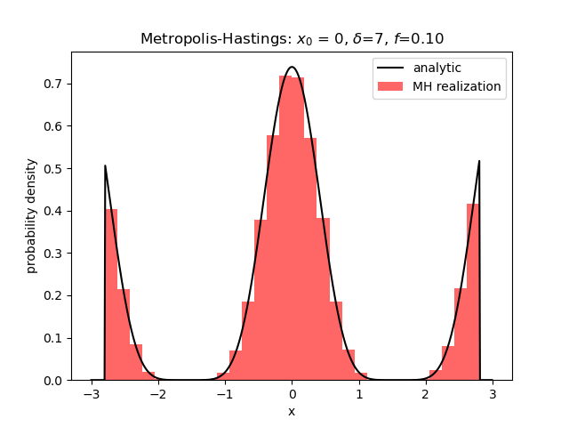
In this case, the distribution has a large central hump or mode and two truncated wings. The best results came from a starting value of $x_0$ at or near zero and a large value of $\delta$.
Lowering the value of $\delta$ leads to the algorithm being trapped in the central peak with no way to cross into the wings.

Finally, starting in the wings with a large value of $\delta$ leads to a realization that looks like it has the general idea as to the shape of the distribution but without the ability to capture the fine detail.
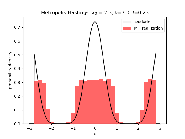
This behavior persists even when the number of trials is increased by a factor of 10 and no immediately satisfactory explanation exists.