Our journey through various Monte Carlo techniques has been rich and rewarding but has been confined almost exclusively to one-dimensional sampling. Even the case of the sunny/rainy-day multi-state Markov Chain (prelude and main act) was merely a precursor to the setup and analysis of the Metropolis-Hastings algorithm that was then applied in one dimension. This month, we step off the real number line and explore the plane to understand a bit of how multivariate sampling works and the meaning of covariance.
To start, let’s imagine that we are measuring the height and weight of some mythical animal, say the xandu of C.S. Friedman’s Coldfire Trilogy. Further suppose that we’ve measured 5000 members of the population and recorded their height and weight. The following figure shows the distribution of these two attributes plus the quantitative statistics of the mean and standard deviation of each.
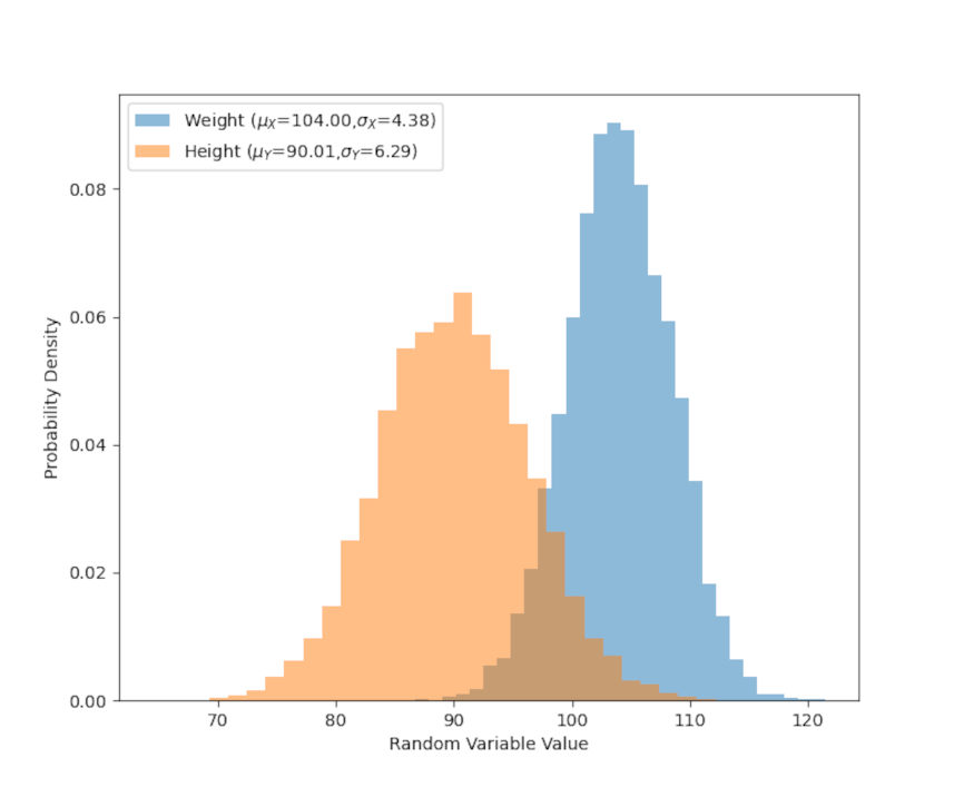
While these statistics give us a good description of the distribution of the weight or the height of the xandu population that don’t say anything about the connection between these two attributes. Generally, we would expect that the larger an animal is the heavier that animal will be, all others things being equal. To better understand the relationship between these two population characteristics, we first make a scatter plot of their weight arbitrarily displayed on the x-axis ($X$ will hereafter be a stand in symbol for weight) and their height along the y-axis ($Y$ for height).
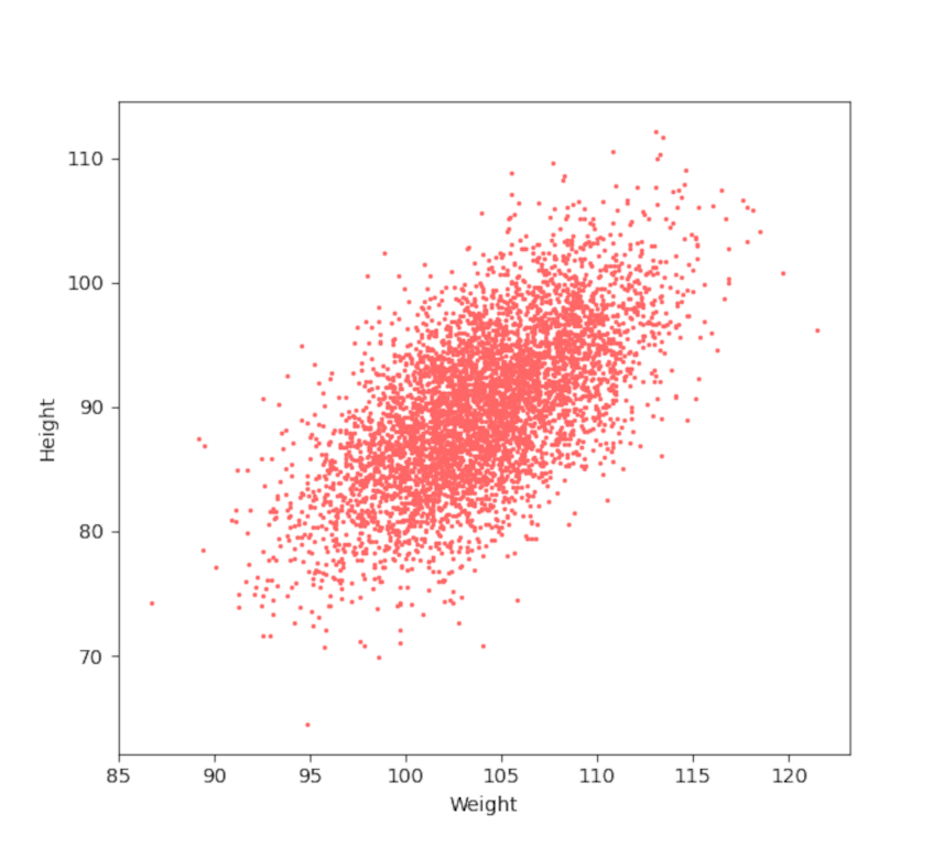
It is obvious that the two attributes are strongly correlated. To make that observation quantitative we first define the covariance matrix between the two series. Let’s remind ourselves that the variance of a set of $N$ values of the random variable $X$, denoted by ${\mathbf X} = \left\{ x_1, x_2, \ldots , x_N\right\}$ defined as
\[ {\sigma_X}^2 = \frac{1}{N} \sum_{i=1}^N \left( x_i – {\bar x} \right)^2 \; , \]
where ${\bar x}$ is the mean value given by
\[ {\bar x} = \frac{1}{N} \sum_{i=1}^N x_i \; . \]
We can express these relations more compactly by defining the common notation of an expectation value of $Q$ as
\[ E[Q] = \frac{1}{N} \sum_{i=1}^N q_i \; , \]
where $Q$ is some arbitrary set of $N$ values denoted as $q_i$. With this definition, the variance becomes
\[ {\sigma_X}^2 = E \left[ (X – {\bar x})^2 \right] \; . \]
The covariance is then the amount the set $X$ moves with (or covaries) with the set $Y$ defined by
\[ Cov(X,Y) = E \left[ (X – {\bar x}) (Y – {\bar y} ) \right] \; .\]
Note that the usual variance is now expressed as
\[ {\sigma_X}^2 = Cov(X,X) = E \left[ (X – {\bar x}) (X – {\bar x}) \right] = E \left[ (X – {\bar x})^2 \right] \; , \]
which is the same as before.
There are four unique combinations: $Cov(X,X)$, $Cov(X,Y)$, $Cov(Y,X)$, and $Cov(Y,Y)$. Because the covariance in symmetric in its arguments $Cov(Y,X) = Cov(X,Y)$. For reasons that will become clearer below, it is convenient to display these four values in the covariance matrix
\[ {\mathcal P}_{XY} = \left[ \begin{array}{cc} Cov(X,X) & Cov(X,Y) \\ Cov(Y,X) & Cov(Y,Y) \end{array} \right] \; , \]
where it is understood that in real computations the off-diagonal terms are symmetric.
The computation of the covariance matrix for the data above is
\[ {\mathcal P}_{XY} = \left[ \begin{array}{cc} 19.22857412 & 17.51559386 \\ 17.51559386 & 39.54157185 \end{array} \right ] \; . \]
The large off-diagonal components, relative to the size of the on-diagonal components, reflects the strong correlation between weight and height of the xandu. The actual correlation coefficient is available from the correlation ${\bar {\mathcal P}}_{XY}$ matrix defined as dividing the terms by the standard deviation of the arguments used
\[ {\bar {\mathcal P}}_{XY} = \left[ \begin{array}{cc} Cov(X,X)/{\sigma_X}^2 & Cov(X,Y)/\sigma_X \sigma_Y \\ Cov(Y,X)/\sigma_Y \sigma_X & Cov(Y,Y)/{\sigma_Y}^2 \end{array} \right] \; .\]
Substituting the values in yields
\[ {\bar {\mathcal P}}_{XY} = \left[ \begin{array}{cc} 1.00000 & 0.63577 \\ 0.63577 & 1.0000 \end{array} \right ] \; . \]
The value of 0.63577 shows that the weight and height are moderately correlated so that about 64% of the variation of the one explains the variation of the other.
With these results in hand, let’s return to why it is convenient to display the individual covariances in matrix form. Doing so allows us to use the power of linear algebra to find the independent variations, $A$ and $B$, of the combined data set. When the weight-height data are experimentally measured, the independent variations are found by diagonalizing the covariance matrix. The resulting eigenvectors indicate the directions of independent variation (i.e., $A$ and $B$ will be expressed as some linear combination of $X$ and $Y$) and the eigenvalues are the corresponding variances ${\sigma_A}^2$ and ${\sigma_B}^2$. The eigenvector/eigenvalue decomposition rarely yields results that are generally understandable as the units of the two variables different but, nonetheless, one can think of the resulting directions as arising from a rotation in the weight-height space.
Understanding is best achieved by using a contrived example where we start with known population parameters for $A$ and $B$ and ‘work forward’. For this example, $\mu_A = 45$ and $\mu_B = 130$ with the corresponding standard deviations of $\sigma_A = 3$ and $\sigma_B = 7$, respectively. These data are then constructed so that they differ from $X$ and $Y$ by a 30-degree rotation. In other words, the matrix equation
\[ \left[ \begin{array}{c} X \\ Y \end{array} \right] = \left[ \begin{array}{cc} \cos \theta & \sin \theta \\ -\sin \theta & \cos \theta \end{array} \right] \left[ \begin{array}{c} A \\ B \end{array} \right] \; \]
relates the variations in $A$ and $B$ to the variation in $X$ and $Y$, where $\theta = 30^{\circ}$. It also relates the mean values by
\[ \left[ \begin{array}{c} \mu_X \\ \mu_Y \end{array} \right] = \left[ \begin{array}{cc} \cos \theta & \sin \theta \\ -\sin \theta & \cos \theta \end{array} \right] \left[ \begin{array}{c} \mu_A \\ \mu_B \end{array} \right] \; , \]
yielding values of $\mu_X = 103.97114317$ and $\mu_Y = 90.08330249$. Note that these are exact values and that the means calculated earlier are estimates based on the sampling.
The exact covariance can also be determined from
\[ {\mathcal P}_{XY} = M {\mathcal P}_{AB} M^{T} \; , \]
where the diagonal matrix ${\mathcal P}_{AB} = diag({\sigma_A}^2,{\sigma_B}^2)$ reflects the fact that $A$ and $B$ are independent random variables and where the ‘$T$’ superscript means the transpose. The exact value is
\[ {\mathcal P}_{XY} = = \left[ \begin{array}{cc} 19.0 & 17.32050808 \\ 17.32050808 & 39.0 \end{array} \right] \; . \]
Again, note both the excellent agreement with what has been estimated from the sampling.
These methods generalize to arbitrary dimension straightforwardly.
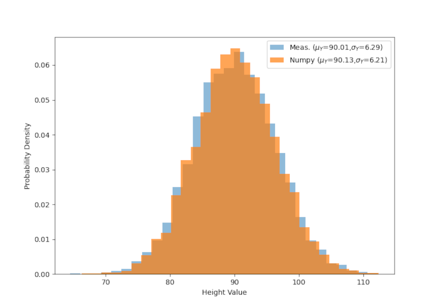
Finally, all of the sampling here was done using numpy, which conveniently has a multivariate sampling method. The only draw back is that it requires knowledge of the exact means and covariances so the above method of mapping $A$ and $B$ to $X$ and $Y$ is necessary. It is instructive to see how well the multivariate sampling matches the method used above in both scatter plot
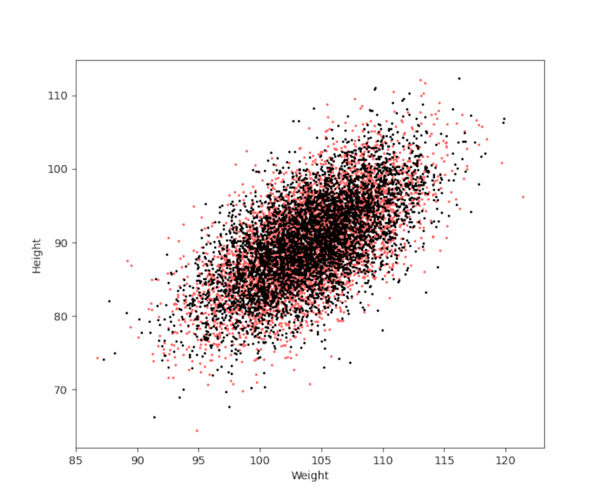
and in the individual distributions for weight
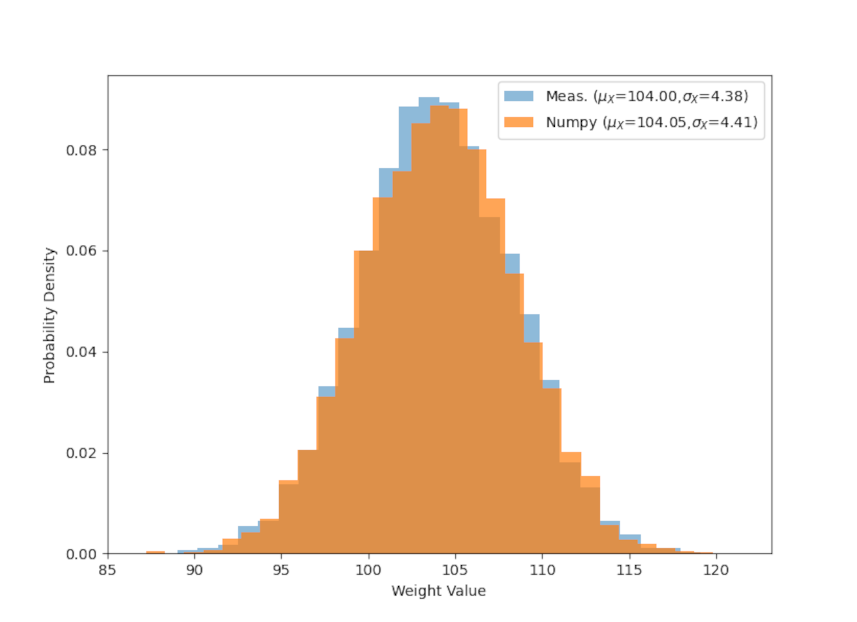
and height