Time Series 2 – Introduction to Holt-Winter
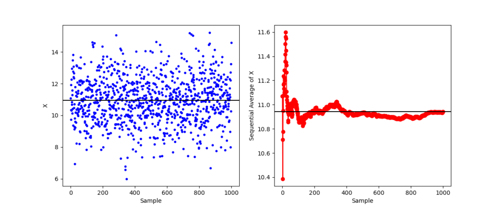
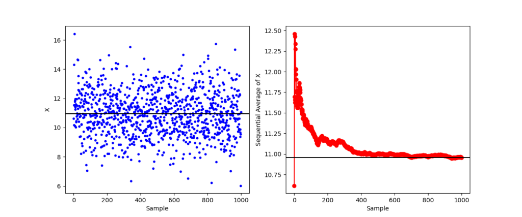
In the last blog, I presented a simple sequential way of analyzing a time series as data are obtained. In that post, the average of any moment $x^n$ was obtained in real-time by simply tracking the appropriate sums and number of points seen. Of course, in a real world application, there would have to be a bit more intelligence built into the algorithm to allow an agent employing it to recognize when a datum is corrupted or bad or missing (all real world problems) and to exclude these point both from the running sums and from the number of points processed.
This month, we look at a more sophisticated algorithm for analyzing trends and patterns in a time series and for projecting that analysis into the future sequential using these patterns. The algorithm is a favorite in the business community because, once an initial ‘training’ set has been digested, the agent can update trends and patterns with each new datum and then forecast into the future. The algorithm is called the Holt-Winter triple exponential smoothing and it has been used in the realm of business analytics for forecasting the number of home purchases, the revenue from soft drink sales, ridership on Amtrak, and so on, based on a historical time series of data.
Being totally unfamiliar with this algorithm until recently, I decided to follow and expand upon the fine video by Leslie Major entitled How to Holts Winters Method in Excel & optimize Alpha, Beta & Gamma. In hindsight, this was a very wise thing to do because there are quite a few subtle choices for initializing the sequential process and the business community focuses predominantly on using the algorithm and not explaining rationale for the choices being followed.
For this first foray, I am using the ‘toy’ data set that Majors constructs for this tutorial. The data set is clean and well-behaved but, unfortunately, is not available from any link discernable associated with the video but I have reconstructed it (with a lot a pauses) and make it available here.
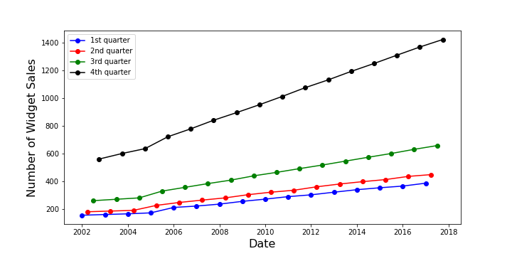
The data are sales $W$ of an imaginary item, which, in deference to decades of tradition, I call a widget. The time period is quarterly and a plot of the definitive sales $W$ from the first quarter of 2003 (January 1, 2003) through the fourth quarter of 2018 (October 1, 2018) shows both seasonal variations (with a monotonic ordering from the first quarter as the lowest to the fourth quarter as the highest)
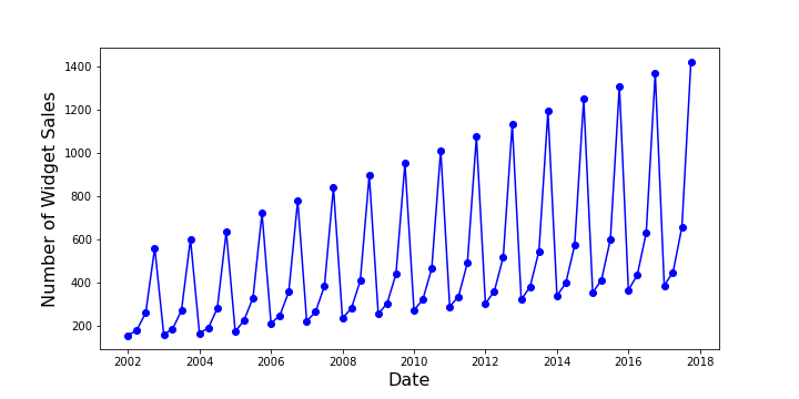
as well as a definite upward trend for each quarter.
The Holt-Winter algorithm starts by assuming that the first year of data are initially available and that a first guess for a set of three parameters $\alpha$, $\beta$, and $\gamma$ (associated with the level $L$, the trend $T$, and the seasonal $S$ values for the number of widget sales, respectively) are known. We’ll talk about how to revise these assumptions after the fundamentals of the method are presented.
The algorithm consists of 7 steps. The prescribed way to initialize the data structures tracking the level, trend, and seasonal values is found in steps 1-4, step 5 is a boot-strap step initialization needed to start the sequential algorithm proper once the first new datum is obtained and steps 6-7 comprise the iterated loop step used for all subsequent data, wherein an update to the current interval is made (step 6) and then a forecast into the future is made (step 7).
In detail these steps require an agent to:
- Determine the number $P$ of intervals in the period; in this case $P = 4$ since the data are collected quarterly.
- Gather the first period of data (here a year) from which the algorithm can ‘learn’ how to statistically characterize it.
- Calculate the average $A$ of the data in the first period.
- Calculate the ratio of each interval $i$ in the first period to the average to get the seasonal scalings $S_i = \frac{V_i}{A}$.
- Once the first new datum $V_i$ ($i=5$) (for the first interval in the second period) comes in, the agent then bootstraps by estimating:
- the level in the first interval by making a seasonal adjustment. Since the seasonal level is not yet known, the agent uses the seasonal value in the previous period in the first interval using $L_i = \frac{V_i}{S_{i-P}}$;
- the trend of the first interval in the second period using $T_{i} = \frac{V_i}{S_{i-P}} – \frac{V_{i-1}}{S_{i-1}}$. This odd looking formula is basically the finite difference between the first interval of the second period and the last interval of the first period, each seasonally adjusted. Again, since the seasonal level is not yet know, the agent uses the seasonal value from the corresponding earlier interval for the first interval of the second period;
- the seasonal ratio of the first interval in the second period using $S_i = \gamma \frac{V_i}{L_i} + (1-\gamma) S_{i-P}$.
- Now, the agent can begin sequential updating in earnest by using all of the weighted or blended averages of the data in current and past intervals to update:
- the level using $L_i = \alpha \frac{V_i}{S_{i-P}} + (1-\alpha)(L_{t-1} + T_{t-1})$
- the trend using $T_i = \beta ( L_i – L_{i-1} ) + (1-\beta) T_{t-1}$
- the seasonal ratio (again) using $S_i = \gamma \frac{V_i}{L_i} + (1-\gamma) S_{i-P}$
- Finally, the agent can forecast as far forward as desired (using $F_{i+k} = (L_i + k \cdot T_i) S_{i – P + k}$. where $k$ is an integer representing the number of ‘intervals’ ahead to be forecasted. There are some subtleties associated with what the agent can do with a finite number of historical levels of the seasonal ratios, so, depending on application, specific approximations for $S_{i – P + k}$ must be made.
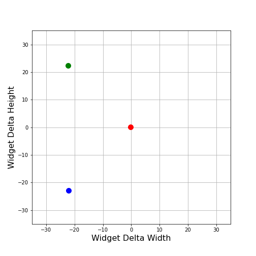
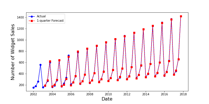
Using the widget sales data, the first 4-quarter forecast compares favorable to the actuals as seen in the following plot.
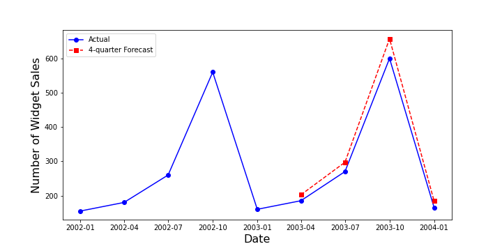
When forecasting only a quarter ahead, as Major herself does, the results are also qualitatively quite good.
Finally, a note about selecting the values of $\alpha$, $\beta$, and $\gamma$. There is a general rule of thumb for initial guesses but that the way to nail down the best values is to use an optimizer to minimize the RMS error between a forecast and the actuals. Majors discusses all of these points and shows how Excel can be used in her video to get even better agreement.
For next month, we’ll talk about the roots of the Holt-Winter algorithm in the exponential smoother (since it is applied to three parameters – level, trend, and seasonal ratio – that is why the algorithm is often called triple exponential smoothing).