Representing Time
Time is a curious thing. John Wheeler is credited with saying that
Certainly this is a common, if unacknowledged, sentiment that pervades all of the physical sciences. The very notion of an equation of motion for a dynamical system rests upon the representation of time as a continuous, infinitely divisible parameter. Time is considered as either the sole independent variable for ordinary differential equations or as the only ‘time-like’ parameter for partial differential equations. Regardless, the basic equation of the motion for most physical processes takes the form of
\[ \frac{d}{dt} \bar S = \bar f(\bar S; t) \]
where the state $\bar S$ can be just about anything imagined and the generalized force $\bar f$ depends on the state and, possibly, the time. By its very structure, these generic form implies that we think of time as something that can be as finely divided as we wish – how else can there be any sense made of the $\frac{d}{dt}$ operator.
Even in the more modern implementations of cellular automata, where the time updates occur at discrete instants, we still think of the computational system as representing a continuous process sampled at evenly spaced times.
The very notion of continuous time is inherited from the ideas of motion and here I believe that Wheeler’s aphorism is on target. The original definition of time is based on the motion of the Earth about its axis with the location of the Sun in the sky moving continuously as the day winds forward. As the invention of timekeeping evolved, items, like the sundial, either abstracted the sun’s apparent motion to something more easily measured, or replaced that motion with something more easily controlled like a clock. Thus time for most of us takes on the form of the moving hands of the analog clock.
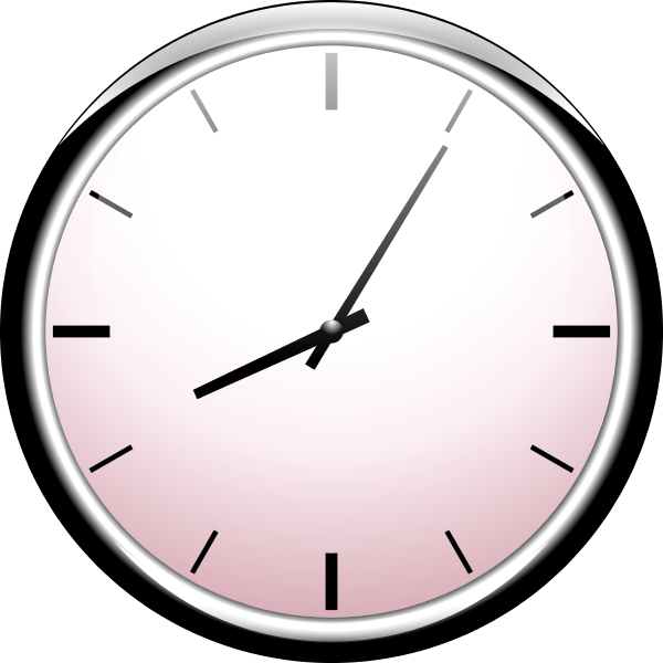
The location of the hands is a continuous function of time, with the angle that the hour and minute (and perhaps second) hands make with respect to high noon going something like $\sin(\omega t)$ where the angular frequency $\omega$ is taken to be negative to get the handedness correct.
But as timekeeping has evolved does this notion continue to be physical? Specifically, how should we think about the pervasive digital clock
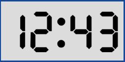
and the underlying concepts of digital timekeeping on a computer.
Originally, many computer systems were designed to inherit this human notion of ‘time as motion’ and time is internally represented in many machines as a double precision floating point number. But does this make sense – either from the philosophical view or the computing view?
Let’s consider the last point first. Certainly, the force models $\bar f(\bar S;t)$ used in dynamical systems require a continuous time in the calculus but they clearly cannot get such a time in the finite precision of any computing machine. At some level, all such models have to settle for a time just above a certain threshold that is tailored for the specific application. So the implementation of a continuous time expressed in terms of a floating point variable should be replaced with one or more integers that count the multiples of this threshold time in a discrete way.
What is meant by one or more integers is best understood in terms of an example. Astronomical models of the motion of celestial objects are usually expressed in terms of Julian date and fractions therein. Traditional computing approaches would dictate that the time, call it $JD$ would be given by a floating point number where the integer part is the number of whole days and the fractional parts the numbers of hours, minutes, seconds, milliseconds, and so on, added together appropriately and then divided by 86400 to get the corresponding fraction. Conceptually, this means that we take a set of integers and then contort them into a single floating point number. But this approach not only involves a set of unnecessary mental gymnastics but is actually subject to error in the numerical sense.
Consider the following two modified Julian dates, represented by their integer values for days, hours, minutes, seconds, and milliseconds and by their corresponding floating point representations
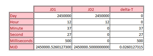
In an arbitrary-precision computation, the sum of $JD1 = JD2 + deltaT$ would be exact but a quick scan over the last two digits of the three numbers involved shows that the floating point representation doesn’t capture the correct representation exactly.
Of course this should come as no surprise since this is an expected limitation of floating point arithmetic. The only way to determine if two times are equal using the floating point method is to difference the two times in question, take the absolute value of the result and to declare sameness if the value is less than some tolerance. Critics will be quick to point out that this fuzziness is the cost of fast performance and that this consideration outweighs exactness, but this is really just a tacit admission of the existence of a threshold time below which one does not need to probe.
Arbitrary precision, in the form of a sufficient set of integers (as used above), circumvents this problem but only to a point. One cannot have an infinite number of integers to capture the smallest conceivable sliver of time. Practically, both memory and performance considerations limit the list of integers in the set to be relatively small. And so we again have a threshold time below which we cannot represent a change.
And so we arrive at the contemplation of the first problem. Is there really any philosophical ground on which we can stand that says that a continuous time is required. Certainly the calculus requires continuity at the smallest of scales but is the calculus truth or a tool? Newton’s laws can only be explored to a fairly limited level before the laws of quantum mechanics becomes important. But are the laws of quantum mechanics really laws in continuous time? Or is Schrodinger’s equation an approximation to the underlying truth? The answer to these questions, I suppose, is a matter of time.