Monthly Archive: April 2016

This post completes a brief three-part study of propositional calculus. In the first post, the basic notions, symbols and rules for this logical system were introduced. The second post dealt with how to prove the validity of an argument. In this context, an argument is a formal manipulation of initial assumptions into a final conclusion using the 10 inference rules. Proofs are highly algorithmic, although usually tricky, and computer programs exist that can workout proofs and determine validity. This post will be devoted to discussion some of the applications of such a decision/inference engine.

The idea of an inference engine making decisions akin to what a human would do is the core notion of an expert system. Expert systems try to encapsulate the problem-solving or decision-making techniques of human experts through the interaction of the inference engine with the knowledge base. Rather than relying on a defined procedural algorithm for moving data back-and-forth, the expert system operators on a set of initial premises using its inference engine to link these premises to facts in its knowledge base. These linked facts then acts as the new premises and the chain continues until the goal is met or the system declares that it has had enough.

There are two different approaches to building the inferential links: forward-chaining and backward chaining.

Forward-chaining works much like syllogistic logic starting from the premises and working forward to the conclusion. The example in Wikipedia is particularly nice in that it demonstrates the method using, perhaps, the most famous syllogism in logic. The knowledge base would have a rule reading something like:

\[ Man(x) \implies Mortal(x) \]

This rule means that anytime the object $x$ is identified as belonging to the set $Man$ it can be inferred that the same object belongs to the set $Mortal$. The inference engine, when given

\[ x = Socrates \; \]

immediately can determine that Socrates is mortal, thus rediscovering in cyberspace the classic syllogism

Backwards-chaining starts with the conclusion and tries to find a path that gets it all the way back to the beginning. Backwards-chaining is often used, to comedic effect, in certain stories in which in order to get something the lead character wants (say Z) he must first acquire Y. But acquisition of Y requires first getting X and so on. Of course, the humor comes when the chain is almost complete only to break apart, link-by-link, at the last moment.

In both cases, the inference rule that is primarily employed is the Modus Ponens which asserts

\[ P \rightarrow Q, P \implies Q \; . \]

It is easy to see that the rise of the expert system explains the importance of propositional calculus.

Now the formal instance of Modus Ponens given above is deceptively simple-looking but can be quite complex when applied to real-world problems. As a result, the actual track record of expert systems is mixed. Some applications have failed (e.g. Hearsay for speech-recognition) whereas other applications have been quite successful (e.g. MYCIN or CADUCEUS for medical diagnoses).

Expert systems were quite in fashion in the late 1980s and early 1990s but their usage has receded from view. It appears that nowadays, they tend to find a place in and amongst other AI tools rather than being standalone systems.

Despite their relegated position in modern AI, expert systems and propositional calculus are still investigated today. One very fun and challenging application is to produce an agent that is capable of playing the game Hunt the Wumpus.

In Hunt the Wumpus, the player finds himself trapped in a dungeon. He can only see the contents of his room and the exits that issue forth. Hidden in the dungeon are pits that will plunge him to a painful death and a Wumpus, a bizarre beast, that will eat the player. Both of these threats are certain doom if the player enters the room in which they are contained. Also hidden in the dungeon is a pile of gold. The player’s goal is to find the gold and kill the Wumpus, thus allowing the player to escape with the riches.

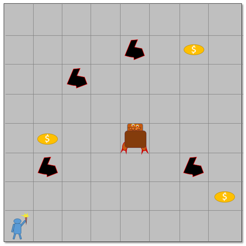
In order for the player to navigate the dungeon, he must depend on his senses of smell and touch. When he is in a room adjacent to a pit, he senses a slight breeze blowing but he cannot tell from where. When he is in a room that is within two of the Wumpus he smells a stench that alerts him that the Wumpus is near. Armed with only one arrow, the player must use his perceptions to deduce where the Wumpus is and, firing from the safety of the adjacent room, must kill the foul beast. Note that this is a variant of the original game – as far as I can tell, all versions are variants and everyone who implements the game tinkers to some minor degree with the game play.

As the player moves around the board, he increases his knowledge base and using propositional calculus, he attempts to win the gold, kill the Wumpus, and escape to tell his tell.

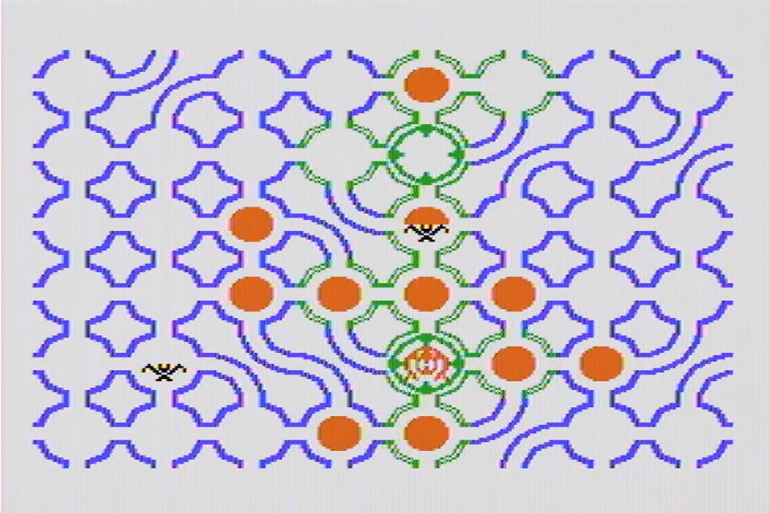
A nice example of the game play available on the TI-99/4A can be found on YouTube. In the following example, the human player has revealed a large percentage of the board.

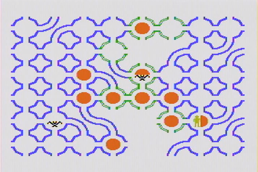
The green colors to the rooms denote the ‘breeze observation’ while the rust color denotes the ‘stench observation’. In this version, there are also bats that, when triggered, transport the player to a random location. These bats, however, rarely seem to activiate and I’ll ignore them.

With a little thought, it is possible to see that there is a pit along the 2nd row from the top and the 5th column from the left. Likewise, the Wumpus in the 6th row and 5th column. The player recognized this and shot appropriately, killing the Wumpus and saving his skin. The following figure shows the game board revealed after th success.

This sort of deduction is relatively easy for the human player once a bit of experience is gained but not so much for the computer agent. As the video below demonstrates, even a relatively simple configuration (without bats and variable topology of the rooms) can be quite challenging.

And so I’ll close with a few final remarks. First, the propositional calculus is a subject alive and well in the AI community. It provides an underpinning for many decisions made by computer agents. Second, the skill of such systems has yet to rival human thought. Maybe it never will… time (and, perhaps the Wumpus) will tell.

The last column introduced the basic structure of the propositional logic consisting of 10 inference rules that manipulated 5 logical symbols: negation $\neg$, conjunction (and) $\land$, disjunction (or) $\lor$, conditional $\rightarrow$, and biconditional $\leftrightarrow$.

The point of the system was to formalize the rules of reasoning so that two difficulties of natural language were eliminated. The first difficulty is that natural language premises (e.g. it is raining) are unwieldy compared to single symbols (e.g. R). The second, and more problematic, difficulty is the ambiguous aspect of natural language.

Suppose that a friend says “I am interested in logic and programming. Could you help me find good websites?” You try to help by doing a web search. How should you frame your search string? Does you friend mean that he is interested in getting hits that deal either with logic or with programming? Or perhaps he only wants sites that discuss both concepts in the same posting. With this ambiguity present, how should the search engine interpret the simple search string ‘logic programming’?

By formalizing and abstracting the objects and rules away from natural language, propositional calculus seeks a clean way of reasoning with algorithmic precision. The line of reasons that infers a set of well-formed formulas (wffs) from an initial set is called, appropriately enough, a proof. The flow of the proof is improved by abbreviating the rules of inference with a 2 or 3 character abbreviation:

1. Modus ponens = MP
2. Negation Elimination = $E\neg$
3. Conjunction Introduction = $I\land$
4. Conjunction Elimination = $E\land$
5. Disjunction Introduction = $I\lor$
6. Disjunction Elimination = $E\lor$
7. Biconditional Introduction = $I\leftrightarrow$
8. Biconditional Elimination = $E\leftrightarrow$
9. Conditional Proof = CP
10. Reductio ad Absurdum = RAA

I don’t find any proofs, except the most elementary ones, particularly easy to figure out and, I suppose, that is the point. If it was easy, there would be no need for the formalism.

As an example (taken from problem 3.31 of Theory and Problems of Logic by Nolt and Rohatyn), consider how to prove the following argument.

$ \neg( P \land Q) \rightarrow \neg P \lor \neg Q $

To recast that in natural language, let P stand for the sentence ‘it is raining’ and Q for ‘the streets are wet’. The argument above says that ‘if it is not true that it is raining and the streets are wet then either it is not raining or the streets are not wet’. This translation is not only a mouthful but, it may seem to some that it is also incomplete. In natural language, the ‘or’ in consequent can be interpreted as being an exclusive or – hat either it is not raining or that the streets are not wet but not both. However, the ‘or’ of propositional logic is the inclusive or that means the assumption is true if the first is true alone, the second is true alone, or both are true. Thus the propositional calculus arrived at a proof that, on the surface, may seem a surprise to the natural language ear.

The formal proof for this argument is given by:

The indentations denote hypothetical proofs within the main body of the proof (this one has 3 Reductio ad Absurdum sub-proofs) and the notation in the last column gives the line number(s) and the rule used to manipulate the wffs.

It is reasonable to ask why go through all this bother. Surely we don’t need formal logic to figure out if it is raining or if the streets are wet. There are several good reasons for studying the propositional calculus but perhaps the most interesting and important is that the system can be programmed on a computer and the rules of inference can be used on problems much harder than the human mind may be willing to deal with.

An interesting example of this is the Tree Proof Generator.

This web-based application allows the user to enter an argument its internal inference engine not only determines the arguments validity but it generates the step-by-step proof.

Now this example may not be particularly motivational until one stops to consider to the scope. Since the well-formed formula can be anything, such a system could solve complex mathematical problems, or go through complicated epidemiological analysis to assist in diagnosing a patient’s illness or in determining the pattern of a epidemic.

In other words, the propositional calculus can be used to make an expert system that can deal with large amounts of data and inferences in a formal way that would be difficult of impossible to people to do unaided.

Next week, I will look at what has been done with such expert agents – in particular with an agent application that attempts to keep a digital explorer from a gruesome cyber-fate.

Propositional calculus is one of the oldest forms of logic.  It lies at the heart of all syllogisms, deductions, inductive inferences, and the like.  It is the system that allows us to deal with logic problems such as determining the truth of the following argument:

or of this argument:

Note that is doesn’t judge the truth or falsehood of the premises (It is raining or it is sunny) or of the conditionals (If it is…), it only judges the truth content of the conclusion based on these assumptions (premises and conditionals).  It won’t know whether or not it is raining, but it will be able to tell me that I am depressed when it is raining (not true – I like the rain) or that I shouldn’t wear a raincoat when it is sunny.  Note also that the system is not equipped to handle syllogism using the quantifiers all, some, or none.  Thus the true syllogism

and the false syllogism

are outside of its ability to evaluate.

Despite these limitations, the system is fairly powerful and can be used in successful applications of artificial intelligence to solve real-world, interesting problems.

Amazingly propositional logic is able to pack a lot of power into a fairly brief amount of symbolism.  The system as a whole consists of 2 objects, 5 expressions that define relations between the objects, 10 rules for manipulating the relations, and 3 helper symbols that act as traffic cops to impose order on the steps.

The simplest object of the system is an atomic proposition, like the statement ‘It is raining’.  This proposition, usually denoted by a single capital letter – ‘R’ for ‘It is raining’.  More complex propositions are built out of the atomic propositions using the 5 logical expressions, subject to certain rules.  Any primitive proposition and all valid compound propositions are collectively known as well-formed formulae (wffs – pronounce ‘woofs’, like the sounds dogs make).  Often wffs are denoted by Greek symbols, like $\phi$ or $\psi$.

The 5 logical expressions denote relations associated with the propositions.  There is one prefix expression, where the expression symbol operators on only one proposition, and 4 infix expressions that link two propositions together.

The prefix expression is the ‘not’ which translates the proposition ‘It is raining’ into the negative proposition ‘It is not the case that it is raining’.  This somewhat more clunky way of expressing the negation (rather than ‘It is not raining’) seems to be preferred since it makes adding or removing a negation as simple as adding or removing the phrase ‘It is not the case that’ to the front of an existing proposition.

The four infix expressions link two propositions together.  These are:

• Conjunction – ‘It is raining’ and ‘It is cold’
• Disjunction – Either ‘it is raining’ or ‘it is sunny’
• Conditional – If ‘it is raining’ then ‘the ground is wet’
• Biconditional – ‘It is raining’ if and only if ‘water droplets are falling from sky’

Since the conjunction, disjunction, and biconditional expressions are symmetric upon interchange of the two propositions (or wffs) there is no special name for the first or second slots.  The conditional, however, requires a sense of cause-and-effect and, as result, the first slot is called the antecedent and the second slot the consequent.  In the conditional ‘If it is raining then I am depressed’, ‘it is raining’ is the antecedent and ‘I am depressed’ is the consequent.

The systems objects and expressions can be summarized as

In addition to the expression symbols, there are a few additional helper symbols that keep things neat.  The first is the ‘implies’ symbol $\implies$. It is sometimes called ‘infer that’ and then is denoted by $\vdash$. Either basically denotes the final conclusion (the output) of the argument.  So the first proposition translates into

where $R$ is the proposition ‘It is raining’ and $D$ is the proposition ‘I am depressed’.  The second set of symbols are the parentheses ‘(‘ and ‘)’ which are used to group terms together to avoid ambiguous expressions such as $A \land B \land C$, which could mean ‘I did A and then I did B and C’ or ‘I did A and B and then I did C’ or other meanings.

The next piece is the rules of inference that allow proper manipulation of one set of wffs into another.  These rules are:

1. Modus ponens: a conditional implies the consequent if the antecedent is true
2. Negation Elimination: $\neg \neg \phi \implies \phi$
3. Conjunction Introduction: $\phi, \psi \implies \phi \land \psi$
4. Conjunction Elimination: $\phi \land \psi \implies \phi, \psi$
5. Disjunction Introduction: $\phi \implies \phi \lor \psi$ for any $\psi$
6. Disjunction Elimination: $\phi \lor \psi, \phi \rightarrow \chi, \psi \rightarrow \chi \implies \chi$
7. Biconditional Introduction: $(\phi \rightarrow \psi), (\psi \rightarrow \phi) \implies \phi \leftrightarrow \psi$
8. Biconditional Elimination: $\phi \leftrightarrow \psi \implies \phi \rightarrow \psi, \psi \rightarrow \phi$
9. Conditional Proof (CP): accepting a proposition $P$ that proves another $Q$ then $P \rightarrow Q$
10. Reductio ad Absurdum (RAA): A contradiction to $\neg \phi \implies \phi$

Note that the truth value of the propositions are assumed to be known from the outset (with the exception of the conditional proof and reduction ad absurdum, where the assumption is made during the course of the argument).  The purpose of the system is to determine the truth of the conclusion based on the truth values of assumptions.  The formal inference rules act as a computer program that transforms input to output.

Next week’s column will apply the Propositional Calculus to prove some interesting outcomes and to show how unexpected inferences can result.  All of that is a prelude to the final, fun application of preventing an AI explorer from dying due to misadventure before he can go ‘there and back again’.

The disciplines of the natural sciences and philosophy enjoy a rich, complicated, and, at times, subtle relationship.  Philosophic pursuits help to guide and inform the scientific enterprise while the phenomena, which science discovers, categorizes, and explains, expands and grounds the philosophic thought.  Nowhere is this interaction more interesting and, perhaps, more important than in the area of knowledge and uncertainty.

Epistemological ideas dealing with what is knowable, unknown, and unknowable have played a large role since the earliest days of philosophy.  In the Platonic dialog The Meno, Socrates puts forward the idea that much (or perhaps all) human learning is really a kind of remembrance of knowledge attained in past incarnations of the soul (anamnesis).  How exactly the cycle starts and what knowledge the proto-soul possesses or whether Plato/Socrates actually worried about an infinite regress is not clear.

Questions of knowledge continue on for thousands of years without much of a change in the focus or tenor until the rise of quantitative scientific methods in the post-Renaissance world.  Almost overnight, there is now a way to discuss three vital components of knowing, at least within the context of physical systems:

• Knowledge characterized by measurement
• Uncertainty characterized by error
• Mathematical description of how the two propagate their influence

These new ingredients are not developed to shed light on ages-old debates but rather to determine just how to deal with these new models of the physical world – differential equations.  In differential equations, man had an operational model for cause-and-effect; a laboratory wherein the ideas of what is known and unknown/unknowable could be made the subject of experimentation.  Nature’s own fabric helped to shape and mold how mankind saw knowledge.

These ideas matured in many different directions subject to need and taste.  The three most interesting ones are:

• Control theory
• Quantum mechanics
• Statistical mechanics

In control theory, the basic notion is one of a state whose evolution is subject to a set of differential equations that describe the influence of the natural environment and the man-made controls used to guide the evolution into a desired behavior.  The physical world is divided into pieces known and unknown.   Generally, the known pieces are considered to be deterministic and the unknown pieces are random.  The random variables are assigned probability distributions that describe what sort of state realizations can occur and how often they are likely to come on the scene.  Sometimes, there is a further division of the random variables as either being aleatory or epistemic.  The former term, aleatory, is best described as saying the randomness is somehow intrinsic to the system being modeled.  In contrast, the latter term, epistemic, refers to randomness that is due to lack of measurement precision.  The errors in the knowledge of the initial state of a system is often thought of as epistemic while the uncertainties in the evolution of the differential equation is often thought of as aleatory.  The distinction being that the initial state knowledge may be improved by better measurements while the evolution model for the system, the so-called right-hand side of the differential equation, will never be able to accurately represent the true dynamics due to random fluctuations in the forces that cause the motion.

Generally, the control system community does delve too deeply into the ontological nature of these uncertainties, contenting themselves with the need to operationally model them.  And this approach is reasonable since it isn’t nearly as important to understand where ‘noise’ comes from as it is to determine how to deal with it.

Nonetheless, the very concept of noise and randomness and the study of how they arise can guide the techniques used to control and mitigate their presence.  This is where the two disciplines in physics, statistical mechanics and quantum mechanics, shine.

These two disciplines are, properly speaking, two sides of the same coin, but it is often convenient to separate out the randomness into two separate bins, one dealing with the quantum nature and the other with the many-particle nature of the system being studies.  Although the terminology is rarely used by physicists, the descriptions of aleatory and epistemic fit these bins nicely, at least at the conceptual level.  However, hard pushing on these concepts will soon show that the divisions are not as clear cut as they might first appear.

First, consider quantum mechanics.  By the very nature of the quantum wave function, the state of a system at any time cannot be determined with infinite precision; so a complete knowledge of conjugate pairs of variables (e.g. position and momentum) is impossible.  In some sense the system is aleatory.  But the evolution of the wave function is mediated by the Hamiltonian, whose nature is considered known.  The state evolution is completely deterministic and the only insertion of randomness comes in the measurement step, where the wave function collapses into an eigenstate of the measurement Hamiltonian.  Thus the measurement process is aleatory but this randomness can be used to an advantage since the initial state of the system can be prepared so that it is perfectly an eigenstate of the measurement Hamiltonian and hence has no state uncertainty.

Statistical mechanics deals with the added complication of having an enormous number of degrees of freedom (e.g. many particles) so that a complete description of the state is practically impossible. (It is interesting to note that not all systems with enormous or even infinite degrees of freedom are intractable; the common field theory – say the wave equation – has an infinite number of Fourier modes that all behave in a describable fashion.)  In classical statistical mechanics, the state of the system is not limited by the uncertainty principle.  So the specification of the initial state is probabilistic only due to our ignorance, thus it is epistemic.  Since tracking separate their individual motions, and hence their interactions, is also intractable, the evolution is subject to ‘noise’ but of an epistemic nature as well; since in principle, if the individual states could be tracked (e.g. on a computer), then complete state knowledge would be possible.

Statistical mechanics becomes richer when combined with quantum mechanics.  The initial state of the system can be statistically distributed across multiple eigenstates.  For example, 10 percent of the system can be in one quantum state while 90 percent in another.  The density matrix formalism is designed to handle the case where epistemic uncertainty is layered on top of aleatory uncertainty.

All this is well and good but things become complicated when these concepts are pushed to their logical boundaries by asking some ontological questions about the nature of uncertainty.  The most intriguing question deal with the boundary between the epistemic and the aleatory.  Many researchers are fascinated with the idea that the aleatory uncertainty of quantum mechanics may give way to hidden variables, pilot waves, and the like.  The unspoken goal is eliminate or, otherwise, get around the uncertainty principle.  But the more interesting question flows the other way.  Is our ignorance a physical manifestation of aleatory rather than of epistemic uncertainty?  Buried deep under these distinctions is the notion of a human who can possess knowledge of the physical world; an observer in the language of quantum mechanics.  But no matter how the knowledge possessor is names, it is still a physical object.  Its knowledge is represented by physical patterns of matter and energy.  Its ability to measure and interact are still mediated materially.  So where does the actual boundary lie?  Just how separate is the measurer from the measured?  The answer is, to close with a pun, completely uncertain.

Thinking about other points-of-view is a proven strategy for more clearly defining what a concept is and what it isn’t.  The heart of the Socratic Method involves repeatedly changing perspectives along this line.  Each dialog employs an operational approach roughly rendered as ‘yes, suppose we look at the matter with this definition, what do we find’.   Following this line of questioning diligently and in a disciplined manner strips away more of the accidentals and allows a sharper picture to emerge of the essential nature of the idea in question.

Such an approach is also useful for sharpening the thinking involved in modeling physical or mathematical objects.   Steps forward in science, particularly physics, comes about often from a cleaner definition of just what some primitive object involves.

Oddly enough, I had the good fortune to be involved in two separate and unrelated discussions this past week about the essential natures of the points-of-view used to describe the physical world, which, in the physical sciences, are always referred to as reference frames or coordinate systems or some closely similar phrasing.   The resulting dialogs certainly helped me to see better what the physical sciences really know about frames and systems of reference.

To set the stage, a disclaimer is in order.  As far as I can tell, there is no universal agreement about how to define a reference frame, or how, exactly, it differs from a coordinate system and the associated measurements.  This lack of uniform definition points to some deep issue – either epistemological or ontological – about the nature of space and time and how humans perceive these things.   One part of the reason seems to be that the operational concepts are so primitive that we have only a basic notion, in many cases, of how to describe it.  I liken it to being able to drive a car or ride a bike but yet be unable to describe how to do these things to someone who can’t.  But I think that there is an even bigger reason that speaks to how we divide the world up into categories and how we identify the essentials from the accidentals.

To make this last point clearer, let me concretely discuss my definitions of reference frame and coordinate system and then point out how one may logically use these definitions to come up with something akin to a contradiction.

A reference frame is a physical object possessing a point-of-view.  The prototype is the human being so defined to have the essential parts of a set of limbs to move about, eyes to look, a mind/brain to process, a mouth to speak the results, and ears to listen.  Even when physics speaks about inanimate objects there is, lurking in the background, the notion of what an observer would see were he a disembodied spirit moving along with or sitting upon the object (such is the nature of our imaginations and how we understand the world).  A convenient abstraction is that a reference frame is any object that has a definite place, which possesses three (independent) directions that it can use, in combination, to point at something, and which has some measure of scale.

Now suppose something of interest comes into this objects field-of-view.  As a reference frame it can point towards the object and can denote how far away the thing of interest is.  By convention, our primitive reference frame object will adjust the length of the direction to the thing of interest, making the length of the arrow along the direction longer or shorter in proportion to the distance. Thus we have defined a traditional position vector with respect to our primitive reference frame.

Note that the notions of direction and distance are also primitive concepts with no easy way to define them in terms of other, simpler things.  Also note that there are no names for the directions yet nor is there any developed idea of how to specify these directions or distances mathematically.

The next step is to remedy this short coming because being able to measure and compute and reproduce values are vital ingredients to understanding the world.  The remedy involves giving the primitive reference frame basic measuring tools.  For this discussion, the ruler, the clock, and the protractor will suffice and the generalization to more sophisticated modes shouldn’t be too hard.

Using only rulers, we can decorate the primitive reference frame with a set of planes, each possessing a ruled grid of lines and spaced with a known distance.  One such configuration is shown below.

The thing of interest is then specified by the labels specifying on which plane and within which cell is it located.  Other objects can be as deftly located and thus we arrive at a coordinate system – an instance of the Cartesian coordinate system to be precise.

Two important things are worth noting.  First, in this scheme, the reference frame possesses the coordinate system – we’ll return to this point below.  Second, the coordinate system is arbitrary.  The planes shown above were oriented so that their edges coincide with the reference frame directions but this choice is no better or worse (at least philosophically) than any other.

Indeed, the whole idea of using planes, regardless of alignment, can be abandoned altogether.  Instead, we could have chosen to use concentric spherical shells of different radii with great circles and latitude lines (taken as primitive notions) drawn on them.  The protractor is now our tool of choice and the result is the spherical coordinate system.  One such shell of one such instance is shown below.

In terms of these shells, the location of the thing of interest would be specified by stating on which shell it lies and by giving the great circle and latitude lines on which it lies.  Of course the orientation of the great circles and latitude lines are as equally arbitrary as the alignment of the planes pictured above.

The whole scheme holds up just fine as long as it is being used operationally.  The trouble comes when one starts examining it closely with an eye to first principles (yet another point-of-view).   Several annoying questions come up which bring into doubt the underlying consistency of the scheme.  Some of these are:

• How can the reference frame have a notion of direction and length without first having some notion of how to measure angles and lengths? In other words, which comes first, reference frame or coordinate system?
• What objects are used to find the position and orientation of the first object – are they not also reference frames? There is a Machian idea buried here but no time to worry about that now.  It suffices to point out that this ambiguity leads to the perpetual confusion between active and passive rotations.

One might also pose the following question.  Since coordinate systems also objects in their own right, with directions determined by lines of constant coordinate value, can’t they also be used as reference frames.  My answer to that question is a guarded no.  Cartesian coordinates really don’t really have an origin that matters – they are really an affine space – so they aren’t quite the same type of object as the primitive thing we attached directions and an origin to.  This observation is also not very solid since the spherical coordinate system has to have an origin upon which the spherical shells are centered.  Even this requirement doesn’t prevent it the origin from shifting, it just makes the algebra much harder and since most everyone goes back to Cartesian coordinates to compute it isn’t a strong point.

More troubling is the observation that some origins are devoid of a physical object.  For example, the barycenter of two equal mass objects separated by a distance great enough that they don’t touch is located in the empty space between them.  Nonetheless, scientists are quite happy to use this mathematical construction as an origin of a reference frame.

So in the final analysis we are left with two basic conclusions.  First, it is no wonder that there is no uniformly, accepted definition of the basic terms of reference frame and coordinate system.  In some sense they are tightly interconnected and too primitive to define precisely.  As long as any scheme works (i.e. give the right numbers) it is operationally sound if not totally logically so.  Second, by studying this thorny problem, we can get some insight into just what is knowable and explainable.