English is a notoriously difficult language to spell and pronounce.  If it challenges the organic learners ability to grasp and communicate it more than doubly so is a source of frustration for the programmer trying to teach bits of silicon, metal, and plastic to appear that they speak naturally.

A famous demonstration of the problems readily encountered in today’s lingua franca, attributed to William Ollier Jr., is the spelling of fish as “ghoti”.  The proper pronunciation of this awkward looking sequence of letters strikes many people as something like “goatey”, an adjective that could be used to describe a thing with the essence or behavior of a the goat.  But Ollier argues for the fish phonetic as follows:

• the letters ‘gh’ are to be pronounced as they are in the word enough
• the letter ‘o’ is to be pronounced as it is in the word women
• the letters ‘ti’ is to be pronounced as it is in the word nation.

Short, simple, and eminently confusing!

Ollier’s first donor word comes from a delightfully ridiculous family of words all sporting the ‘ough’ combination of letters and all having subtly or radically different pronunciations.  Consider the following list:

• bough – a part of a tree; pronounced as [bou]
• bought – the past tense of to buy; pronounce as [bôt]
• cough – an action of the mouth and lungs; pronounced as [käf]
• dough – a mixture of water and flour used in baking; pronounced as [dō]
• enough – just the right amount of a required thing; pronounced [iˈnəf]
• through – to past into and beyond; pronounced [THro͞o]

This list contains six distinct pronunciations for the same four letter combination, representing an astonishing gain of nearly two distinct pronunciations per letter, most likely the greatest variability in the English language, possibly the world.  And it is by no means exhaustive (even if putting it together exhausted the writer). And there are a host of other ‘ough’ words that didn’t make onto the list simply because they offered nothing new.

For example, consider that fought, ought, sought, thought all rhyme with bought and bring nothing new to the list even if they bring headaches to people learning the English tongue.  Similarly, ‘ough’ in drought sounds the same as it does in bough despite the fact that trees need water (or perhaps because of it).  Likewise, though’s similarity to dough consigns it to a mere mention in this paragraph rather than a place of honor (or is it shame) within the bullets above.  And it is tough that tough and rough weren’t unique enough to make the cut.

But perhaps the most interesting no-show on the list is slough.  This word is two-faced having two quite different sounds depending on whether it is a noun or a verb:

• slough – a swamp or mire; pronounced [slou, slo͞o]
• slough – to shed or cast off; pronounced [sləf]

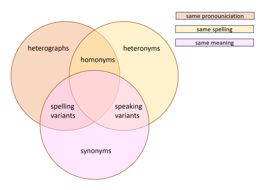
This example is, by no means unique.  English is just brimming with curious words that lie in wait trying to trick the speaker.  There are the heterographs that have the same pronunciation but have different spellings and meanings.  A particularly sinister example is the set of to, too, and two.  There are the homonyms that share both the same pronunciation and spelling but also mean different things.  The clause, the rose rose to glory in the garbage dump, is a fine example.  Together the heterographs and the homonyms form the set of homophones; words that are pronounced the same but which mean different things (regardless of spelling).  Homonyms are also often called homographs, thus serving to bring us to the next category, the synonyms; words with different spellings and pronunciations but which have the same meaning.  Two closely related categories that seem to have no official designation are the spelling variants and the speaking variants. Into the latter go all those weird words like color and colour, saber and sabre, and normalize and normalise.  In the latter category, one finds words like often, in which the speaker may include or omit the ‘t’ sound.

All of these categories can cause problems to speakers, natural and artificial though they may be.  But no category seems to engender as much confusion and consternation as the heteronyms.  Some of the classic examples that fall into this category are:

• bass the musical instrument ([bās]) and bass the fish ([bas])
• minute the unit of time ([ˈminit]) and minute adjective describing size ([mīˈn(y)o͞ot])

Together the heteronyms and homonyms make up the homographs; words with different meanings but the same spelling (regardless of pronunciation).  The following Venn diagram (based on the one in the Wikipedia references) helps one keep score.

Heteronyms are particularly problematic for computer-generated readings of the written word because context changes the pronunciation and meaning in a way that seems hard to find solid rules that work in all instances.

Consider the ridiculous sentence:

Both instances of bass are nouns but it seems clear that the musical instrument can’t be the subject of any sentence, so maybe a programmer can write a rule to accounted for this case or, since it is unlikely that the previous sentence will show up in anything worth writing specialized code to handle, maybe it is ignored altogether.

The sentence:

may be an entirely different story.  There is a reasonable chance that a sentence containing both the noun and adjective form of minute will be written and the word order in the sentence is unlikely to indicate which is which in nearly all cases.  Still the local association of the article a just before the noun form and the occurrence of the noun fraction just after the adjective form may be enough of a pattern to write a rule.

And then there are the voluminous list of noun-verb heteronyms, a sample of which are listed here (for a full list of two-syllable examples):

• Address and address
• Bow and bow
• Buffet and buffet
• Desert and desert
• Dove and dove
• Lead and lead
• Present and present
• Project and project
• Row and row
• Slough and slough
• Tear and tear
• Wind and wind

Writing rules for a machine to naturally speak any sentence with any of these is difficult.  In some cases the word order makes it easier. For example:

guarantees that the subject (he) will be followed by the verb form of bow rather than the noun form.

But other sentences are not so obvious.  Consider these sentences involving the very treacherous word tear, which is a sort of palindrome of noun-verb heteronyms since the [ter] and the [tir] form can be both a noun and a verb.

and

Definitely more difficult, but perhaps doable by scanning the sentence for the helper verbs like will and to.

But the fun doesn’t stop there.  Consider the following command.

Is this a command telling an unidentified person to hand over where he lives or to give a speech to an audience.  There is simply no way of knowing without comprehending the rest of sentences around it.

And there you have, a brief but bewildering dip into what makes learning English a tricky  enterprise. A relatively small set of rules may cover a majority of sentences encountered but to get to fluency an enormous number of special cases and exceptions must be mastered, some of which required a non-local analysis of the text to ensure correctness.  And while teaching a machine to read and speak English aloud is definitely a noble goal for the computer scientist (and especially beneficial for the seeing-impaired) it is one that is likely to come with a whole host of frustrations for year to come. It amazing that any of us can communicate with each other at all.

The year was 1995.  A short-lived and largely unnoticed television show premiered on Fox from March to May of that year.  The show centered around a young woman named Sydney Bloom (played by Lori Singer, who played the role of Cassandra in Warlock), whose father bequeathed her a strange ability.  She was able to enter VR.5, the fifth level of virtual reality, which consisted of her entering with total perception into a cyberspace world that sported realism that matched our own day-to-day reality.

The premise and promise of the show was that a fully immersive digital world was just around the corner.  All that was needed was the familiar trappings of eye-gear, power-glove, computer, and cheesy special effects.  Those modest ingredients allowed her to totally connect with a different reality or, at least, another facet of our reality.

Just a scant three years earlier, the entertainment industry subjected the film-going public to the cringe-worthy spectacle that was the horror movie The Lawnmower Man.  Loosely based on a Stephen King movie, the story follows the tragedy that ensues when a scientist (played by Pierce Brosnan) attempts to boost the brain power of a developmentally challenged man (played by Jeff Fahey) through a combined use of drugs and virtual reality.

Here we see a fairly early representation of tactile suits that are designed to simulate the sense of touch, as well as the concepts of an avatar to represent one’s persona in the virtual world and the reoccurring theme of megalomaniacal behavior brought on by unfettered cyber-license.

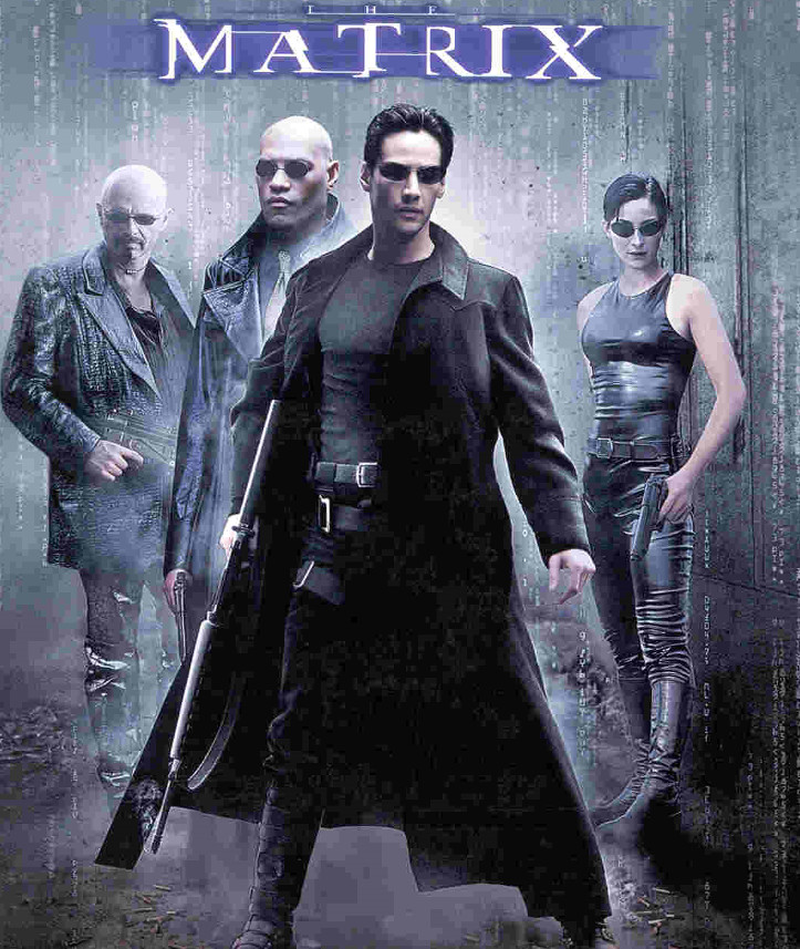
Without a doubt, the most esteemed member of all virtual reality stories must be The Matrix.

Premiering in 1999 under the shadow of The Phantom Menace, the first Star Wars movie in over 15 years, The Matrix was largely overlooked in the months leading up to its release, but the public reception of its storyline and the philosophical questions that it raised made it a classic of American film.  It set the bar for what virtual reality would mean in the science fiction genre, and the tropes, styles, and themes that the entire trilogy used continue to shape VR storytelling to this day.

During the 1990s, it seemed that everywhere you looked the concept of a totally encompassing virtual reality was a narrative staple in almost every type of tale.  Even an entire episode of Murder She Wrote, was devoted to it as a vital clue to solving a crime.  And it isn’t hard to see why VR as a story element showed up in so many places; the concept was flashy and popular and the alternate reality it represents is, at its heart, exactly what storytelling is about – exploring the ‘what ifs’ and ‘what may have beens’ of life.

But the actualization of VR in real life has fallen far short from the promise of these tales.  Like stories involving space travel and artificial intelligence before it, it is far easier to imagine a far-off future of our hopes than it is to realize the more modest goals that we can achieve.  All of these are instances of intoxication fantasies where the mind constructs an idealistic and totally unachievable future by completely disregarding cold, hard facts.

Fortunately, there are realists who are quite willing to redirect ideas and effort to a future that is not only achievable but actually useful.  Space travel doesn’t take us boldly where no man has gone before but it does let us examine land usage, water pollution, and habitat change from a global vantage point.  It connects distant points on the globe, helps us to remain found (rather than being lost), and make instantaneous communications a reality.  AI no longer means machine sentience with all the dreams of utopia and all sinister overtones of dystopia but rather smart agents that act in specific circumstances and within a well-defined realm of applicability faster and more reliably than can a human.  Modern AI techniques help us to make smarter use of limited resources, connect disparate things together to make informed decisions, and help us manage the ever-increasing scale of modern technological life.

Likewise, it seems that VR is moving away from the pipe dream of total immersion and towards a future where the digital supplements the actual.  A panel I attended at Dragon Con a few years back presented an excellent application of augmented reality.  Imagine you are a network engineer and there is a problem with an onsite telecommunications system of one of your customers.   Despite your expertise, qualifications, and certifications, if you’ve never seen the client’s telecom closet, which may look a lot like this,

it will take you some time just to grasp where each blue cable is going to or coming from before you can even begin to troubleshoot which ones are at the root of the problem.  The network topology may be correctly documented on the appropriate diagrams but wading through all the details, trying to match up some lines on a piece of paper to a real world length of cable in order to find the one circuit that you believe is the culprit is a long, tedious process.  Now suppose that instead of a static network diagram, you are able to done VR goggles that overlay portions of the network diagram over top of the image of the real thing that is in front of your eyes.  Suddenly you have a live, heads-up display to assist your navigation of the network design that rivals the best tutorials that videogames have to offer.  This use of VR is so promising that Koch Industries is touting it in their newest press release.

There are other equally humdrum but interesting applications.  One that is particularly near and dear to my heart is the use of VR to explore complicated 3D data.  I had a recent occasion to look at the tangled magnetic field patterns that arise in certain geophysical situations, and a few minutes in VR space did a lot more for my understanding than months of looking at 2D slices and projections.

So, maybe there is a future after all for VR, just not the one that futurists and science fiction writers envisioned.  Never would have seen that coming.

This month’s installment will be the final column of this series on the chaos game.  As befitting any swan song, this ending should be artistic and dramatic and awe-inspiring.  Unfortunately, the chaos game isn’t really dramatic or awe-inspiring – at least for most people – but it can be quite artistic.  The patterns that can be produced can be quite beautiful and pleasing to the eye.  So, this article will be mostly a tour of our local digital museum displaying the various works of art that one can produce using either the code heretofore presented or with some minor modifications.

The first entry in our tour is the Barnsley fern, which is a self-similar structure invented by Michael Barnsley to resemble the black spleenwort fern.  There are four entries into the set affine mappings that comprise the game:

barnsley_fern = np.array([[0.01,   0,      0,    0,0.16,0,   0],
                          [0.86, 0.85,  0.04,-0.04,0.85,0,1.60],
                          [0.93, 0.20, -0.26, 0.23,0.22,0,1.60],
                          [1.00,-0.15,  0.28, 0.26,0.24,0,0.44]])

When run through the chaos game, a remarkably pleasing fern frond is found (alliteration, a sure sign of class).

Surprisingly, one of the affine mappings in the table has only a 1 percent chance of being selected. Modification of the first entry in the table of affine mappings from 0.01 to 0.2,

barnsley_fern_2 = np.array([[0.20,   0,      0,    0,0.16,0,   0],
                            [0.86, 0.85,  0.04,-0.04,0.85,0,1.60],
                            [0.93, 0.20, -0.26, 0.23,0.22,0,1.60],
                            [1.00,-0.15,  0.28, 0.26,0.24,0,0.44]])

thus increasing the probability of using the first mapping at the expense of the second, results in a slightly less luxurious, or mangier but, nonetheless, quite similar frond.

This result strongly supports the conclusion from the last post that the chaos game operations on this set of affine maps seems to be quite stable against changes.  Play of this kind also opens the door to the idea of a meta chaos game where the exact set of affine maps used at any iteration is either subjected to small random variations or is picked from a larger set.  In the latter case, one can imagine a meta algorithm selecting between the barnsley_fern and barnsley_fern_2 tables for each frond as part of a larger plant or switching between the two at random.  Perhaps this type of numerical experiment will form the subject of a future column.

But now back to the tour.

Other mathematicians, professional and amateur alike, have played with the set of affine mappings to create similar plant-like results.  An interesting example, called here the Flatter Fern, has as its set of affine mappings

flatter_fern = np.array([[0.02,0,0,0,0.25,0,-0.4],
                         [0.86,0.95,0.005,-0.005,0.93,-0.002,0.5],
                         [0.93,0.035,-0.2,0.16,0.04,-0.09,0.02],
                         [1.00,-0.04,0.2,0.16,0.04,0.083,0.12]])

Using this table in the chaos game gives

As in the previous case, the structure is self-similar but each of the leaf groups is thinner and straighter than in the Barnsley fern.

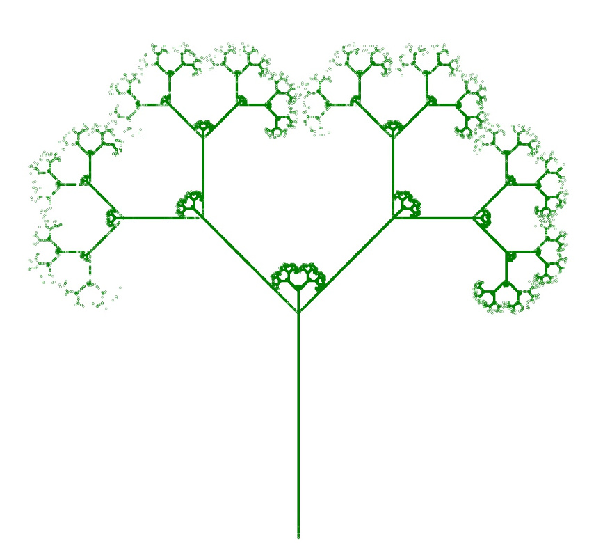
Keeping with the botanical theme, another fan favorite is the Fractal Tree.  Its set of affine maps is

fractal_tree  = np.array([[0.05,   0,    0,    0, 0.5, 0,  0],
                          [0.45,0.42,-0.42, 0.42,0.42, 0,0.2],
                          [0.85,0.42, 0.42,-0.42,0.42, 0,0.2],
                          [1.00, 0.1,    0,    0, 0.1, 0,0.2]])

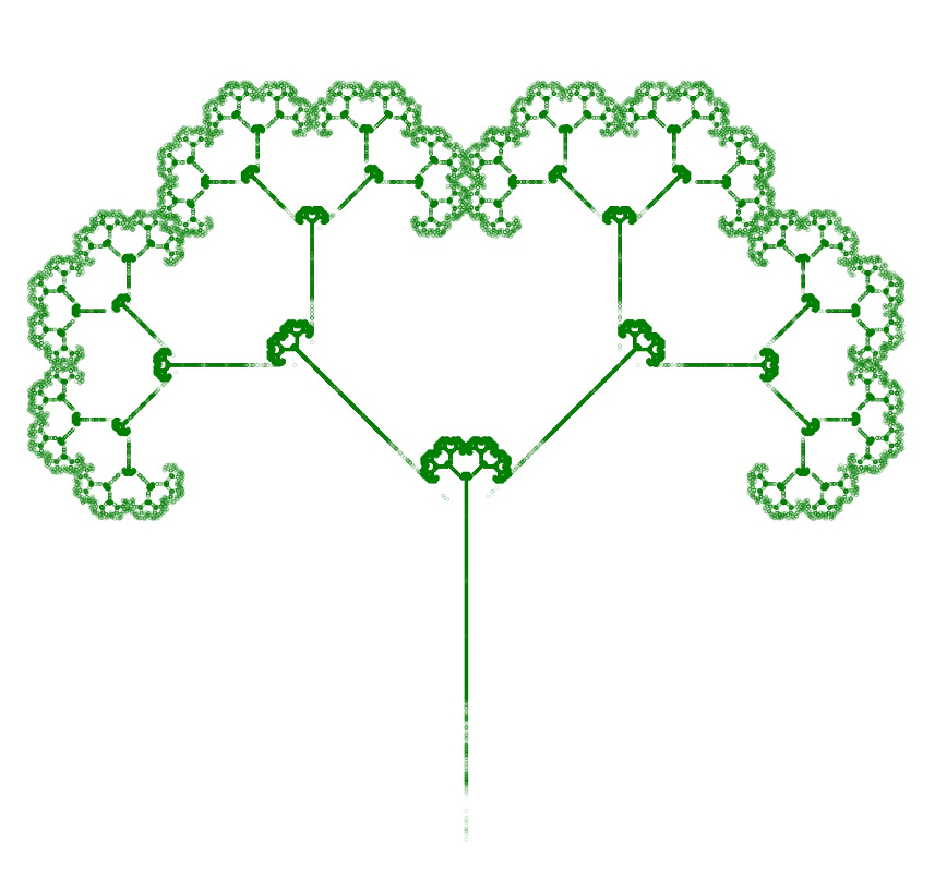
Running the chaos game with this table gives something that looks more like broccoli than it does a tree.

Once again, one can play with the stability of the game by adjusting the relative probabilities.  By upping the probability of the first map of the set from 0.05 to 0.25, giving the following table

fractal_puff  = np.array([[0.25,   0,    0,    0, 0.5, 0,  0],
 [0.45,0.42,-0.42, 0.42,0.42, 0,0.2],

[0.85,0.42, 0.42,-0.42,0.42, 0,0.2],

[1.00, 0.1,    0,    0, 0.1, 0,0.2]])

the chaos game produces a Fractal Puff

which suggests that the outer edge is soft, fuzzy, and worn away.

In the next wing of the museum awaits a curious set of geometric shapes.  The one we will examine in detail is the Square, whose set of affine maps is displayed in the following table.

square  = np.array([[0.25,0.5,0,0,0.5, 1, 1],
                    [0.50,0.5,0,0,0.5,50, 1],
                    [0.75,0.5,0,0,0.5, 1,50],
                    [1.00,0.5,0,0,0.5,50,50]])

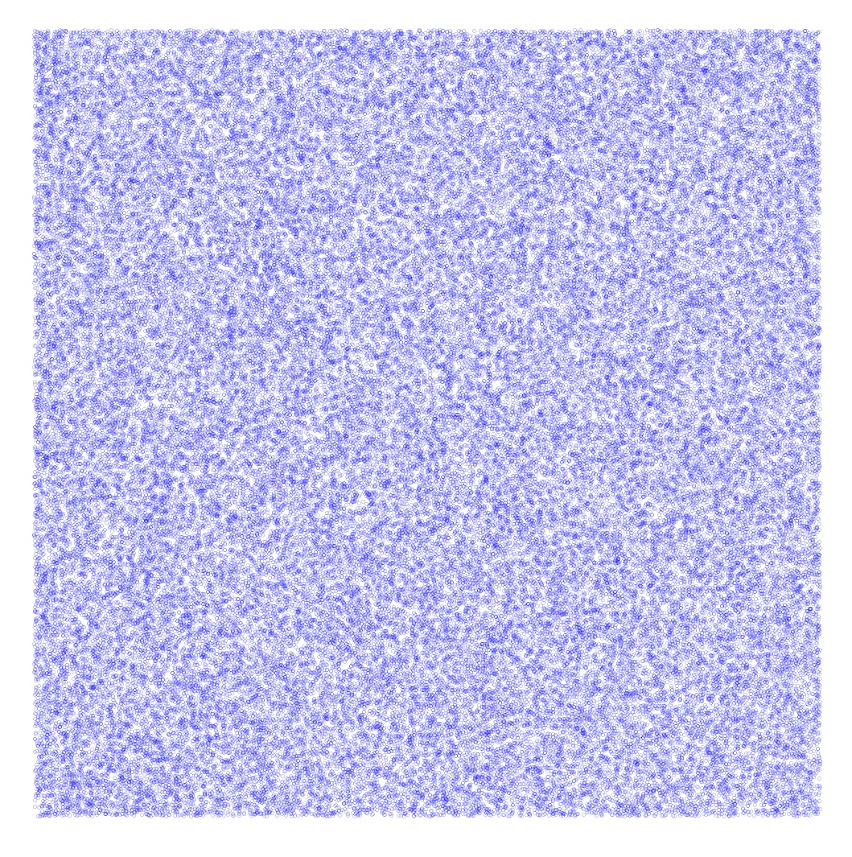
In this case, running the chaos game with this table results in a uniformly filled region.

The trick to making a fractal appear is to restrict the selection of the vertex so that the same vertex cannot be picked in a row.  The easiest modification to the code used in these explorations is to create a new transformation function

def Transform2(point,table,r,prev_N):
    x0 = point[0]
    y0 = point[1]
    for i in range(len(table)):
        if r <= table[i,0]:
            N = i
            break
    if N != prev_N:
        x = table[N,1]*x0 + table[N,2]*y0 + table[N,5]
        y = table[N,3]*x0 + table[N,4]*y0 + table[N,6]
    else:
        x = np.NaN
        y = np.NaN
    
    return np.array([x,y]), N

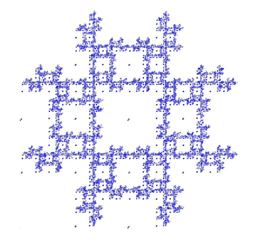
that is aware of the previous vertex (the variable prev_N) and returns a null result for the new point.   Testing the return value keeps the ‘bad’ point out of the results giving the following pattern

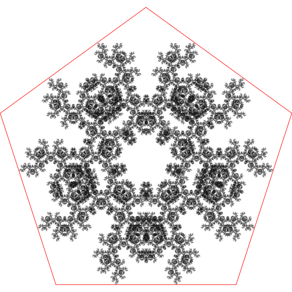
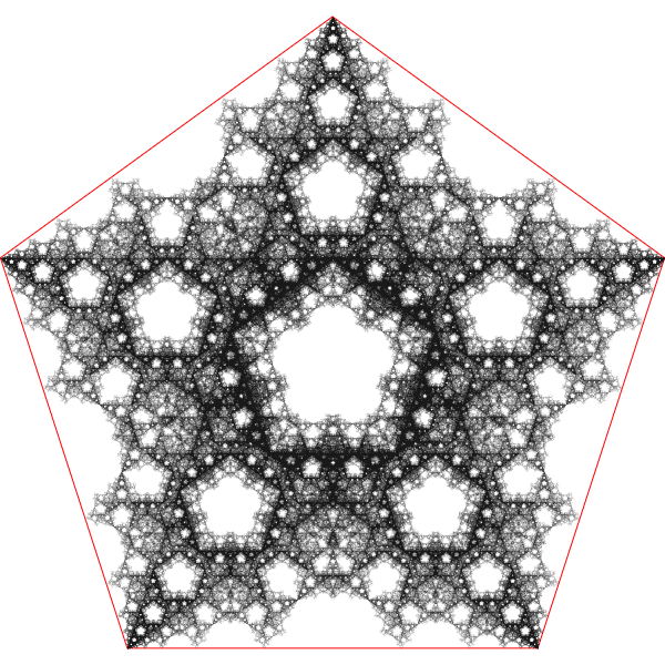
The Wikipedia article on the chaos game, has a stunning gallery of geometric shapes that result from by similar types of rules restricting vertices.  Particularly interesting are the pentagon examples by Edward Haas.

The first one, shows the resulting pattern by using an analogous set of maps to the square and restricting the vertex to be strictly different from the one before.

In Haas’s second case, the pattern results from using the same table as his first case, but with the restriction that the new vertex cannot be 1 or 4 places away from the two previously chosen vertices.

While both cases exhibit five-fold symmetry the differences that arise solely due to the restriction on the allowed vertices is startling.

The final exhibit is a mix of the botanical and the geometric.  The Fractal Tree table was used with the vertex restriction rule used with the square.  The resulting Fractal Twig is beautiful in its brutal desolation (always wanted to talk like a snooty, pretentious modern art dealer)

So, it seems as if the sky is the limit in creating digital art using the chaos game.  I suspect we’ve only scratched the surface.

Now having introduced the chaos game and analyzed how a single iteration works, it is worth taking stock of what we actually know.  Clearly the repeated application of the affine map causes points to collect only in certain places in the plane creating the self-similar fractals that are often called the attractors of the map or strange attractors.  We’ve also established what the parameters of the affine map do in the particular case of the Sierpinski triangle, getting a sense of how those parameters map to the rules discussed in the Numberphile video.  But the exact mechanism for why only certain points are hit is based on some specialized mathematics and little intuition is obtained from pursuing the study without a lot of initial effort being devoted to understanding the ‘nuts and bolts’.

So, this post is devoted to an experimental approach to the chaos game that produces the Sierpinski triangle.  Each experiment performed involves changing one or more of the parameters that make up the affine maps used in the game and then observing what happens to the pattern produced.  Doing so will help us understand the stability of the map.

Stability can be defined in numerous ways.  There are definite schools of thought with different interpretations.  For this exploration of the chaos game, I will define two types of stability:  deterministic and stochastic.

Deterministic stability looks to see in what range of parameters does the chaos game yield fractal-like results.  The parameters themselves are chosen at the beginning of the game and remain fixed during its progression.   The idea is to answer such questions as:  How accurate do the parameters need to be?  How many different shapes or patterns result?  How many different types of games are there?

To get a sense of what answers may result and to clarify what is meant by ‘types of games’, consider the investigation detailed in the last post.  As a direct byproduct of understanding a single iteration, the significance of the constant terms $f^{(p)}$ and $g^{(p)}$ used in three Sierpinski affine maps became clear; multiplying these parameters by two gave the coordinates of vertices of the triangle.  The same Sierpinski triangle resulted even if these values were changed.  Thus, the family of all possible values for $f^{(p)}$ and $g^{(p)}$ form an equivalence class where the scale and overall geometry may change but the shape is undeniably a Sierpinski triangle.  I term this equivalence class as a single game.

In contrast, stochastic stability involves regarding the parameters of the affine maps as random variables, which vary at each iteration.  The time history of each random variable forms a unique realization that is different each time the game is played.  This aspect can be quite important because noise can creep into the game in a variety of scenarios.  Computationally, the finite precision floating point representation of the rational numbers in the game are not exact and small errors arise as the game progresses through its iterations.  Physically, an analog of the game in the material world is a messy affair with the parameters of the maps only inexactly realized due to all the small but unmodelled effects.

One possible way of implementing a stochastic game would be to generalize the deterministic expression for a new point $(x,y)$ in the Sierpinski triangle game,

\[ \left[ \begin{array}{c} x \\ y \end{array} \right] = \left[ \begin{array}{cc} 1/2 & 0 \\ 0 & 1/2 \end{array} \right] \left[ \begin{array}{c} x_{current} \\ y_{current} \end{array} \right] + \frac{1}{2} \left[ \begin{array}{c} x_{vertex} \\ y_{vertex} \end{array} \right] \; , \]

(where $(x_{vertex},y_{vertex})$ are the coordinates of one of the three vertices of the triangle, chosen randomly, and $(x_{current},y_{current})$ is the current points coordinates) to a physical system by making the transformation matrix look like

\[ \left[ \begin{array}{cc} 1/2 & 0 \\ 0 & 1/2 \end{array} \right] \rightarrow \left[ \begin{array}{cc} 1/2 + \eta_{11} & \eta_{12} \\ \eta_{21} & 1/2 + \eta_22 \end{array} \right] \; , \]

where the $\eta_{ij}$ are random variables, with some specified moments, reflecting noise that is ubiquitous in the world.

For this post, we’ll content ourselves with exploring deterministic stability for the Sierpinski triangle, looking at what results from changing the values in the transformation matrix and the relative probabilities that each vertex is selected.  In order to facilitate the experiments, each game’s results will be over-plotted (in black) the results from the standard Sierpinski triangle (red).

The first experiment, we’ll change the transformation matrix so that the new point is only moved one third along the line from the current point to the vertex (this was actually suggested in the Numberphile video).  This modification amounts to the following change for the transformation matrix

\[ \left[ \begin{array}{cc} 1/2 & 0 \\ 0 & 1/2 \end{array} \right] \rightarrow \left[ \begin{array}{cc} 1/3 & 0 \\ 0 & 1/3 \end{array} \right] \; . \]

Running the game gives

At first glance, lowering the values in the transformation matrix seems to have simply shrank the scale of the triangle but closer inspection shows that there is a fundamental change in the geometry.  The missing ‘center piece’ is now a squat hexagon instead of a triangle as is more easily seen with the following annotated figure.

This small change has resulted in a new, but closely related game.

Scaling up the values in the transformation matrix from $1/2$ to $3/4$ leads to no discernible structure (with the original triangle now peaking thru in the lower left corner).

This result looks as if scaling the values in the transformation matrix above $1/2$ causes the points to overlap, suggesting that the value of $1/2$ is some sort of divider or separatrix between non-overlapping and overlapping points.  We might expect that a small value above one half, say $0.55$ would begin to blur the Sierpinski triangle by creating a small amount of overlap.  Running the game with this value yields

Some of the overlap regions are highlighted within red circles and the remaining ones can deduced by the symmetry exhibited by this self-similar fractal.

Likewise, a value of $0.45$ produces a triangle where the sub-triangles no longer smoothly join together but where there are gaps.

If this process were to occur in a physical system (and there are certain researchers constructing such systems – see Physicists wrangled electrons into a quantum fractal) then the scales selected in the transformation matrix must stay confined to a relatively narrow range of parameter space ($0.45-0.55$) before the results become so different as to suggest that the system is fundamentally different.  That said, the geometry produced by the game, regarded strictly in a visual sense, is remarkably resilient.  Triangles within triangles result over a fairly wide range of values.

The results of the final experiment show that the game is even much more tolerant to changes in the probabilities that determine how often each vertex is picked.  In the original implementation of the game, each vertex had a $1/3$ chance of being the one selected.  To see how sensitive the game is to changes in this respect, the relative probabilities were adjusted so that one vertex had an 80% chance of being selected while there was only a 10% chance of selecting from the remaining two.  As the figure below shows, the result of this change are to simply ‘ghost out’ the vertices that are less likely.

The conclusion here is straightforward.  The chaos game method of producing the Sierpinski triangle is remarkably stable to a range of deterministic changes in the parameter set.  This robustness makes the chaos game a convenient numerical laboratory for exploring other emergent fractals, some of which we will see in the next post.

Last month’s blog introduced the idea of the chaos game, which is a simple and compact computing method for generating deterministic fractals using a Monte Carlo-like random method.  The central ingredients of the chaos game are an affine transformation of the plane

\[ \left[ \begin{array}{c} x_i \\ y_i \end{array} \right] = \left[ \begin{array}{cc} a^{(p)} & b^{(p)} \\ c^{(p)} & d^{(p)} \end{array} \right] \left[ \begin{array}{c} x_{i-1} \\ y_{i-1} \end{array} \right] + \left[ \begin{array}{c} f^{(p)} \\ g^{(p)} \end{array} \right] \; , \]

which expresses the current point (labeled by the index i) in terms of the previous point (labeled by the index i-1) in terms of known, fixed parameters $\{a^{(p)}, b^{(p)}, c^{(p)}, d^{(p)}, f^{(p)}, g^{(p)}\}$.  The index $p$ is an integer label for the various affine transformations available and is chosen at random at each step, according to some pre-defined probability distribution.  For the Sierpinski triangle discussed in the previous post, $p$ can take on the values (1,2,3) each with probability 1/3.

It is convenient to package all the information into a table with each row corresponding to a one of the affine transformations.  For the Sierpinski triangle, the table is given by

, which is directly translated into the numpy array

sierpinski_triangle = np.array([[0.33,0.5,0,0,0.5, 1, 1],
                                [0.66,0.5,0,0,0.5, 1,50],
                                [1.00,0.5,0,0,0.5,50,50]])

used for simulation (details in the previous post).

The above material, which is a quick recap of last month’s entry, sets the stage for this post, which focuses on understanding how the structures emerge from such a simple set of rules.

A good starting point for that understanding is the Numberphile video on the chaos game

The presenter, a mathematician by the name of Ben Sparks, starts by showing how the chaos game for the Sierpinski triangle is played by examining single iterations performed by hand.   He performs a single iteration by taking the initial point, rolling a six-sided die (yes die is the correct word for the singular – like Sparks that grammatical rule confuses me as well) to randomly pick one of the three vertices, connecting the point to the chosen vertex with a straight line, and then establishing the new point at a distance halfway along that line.

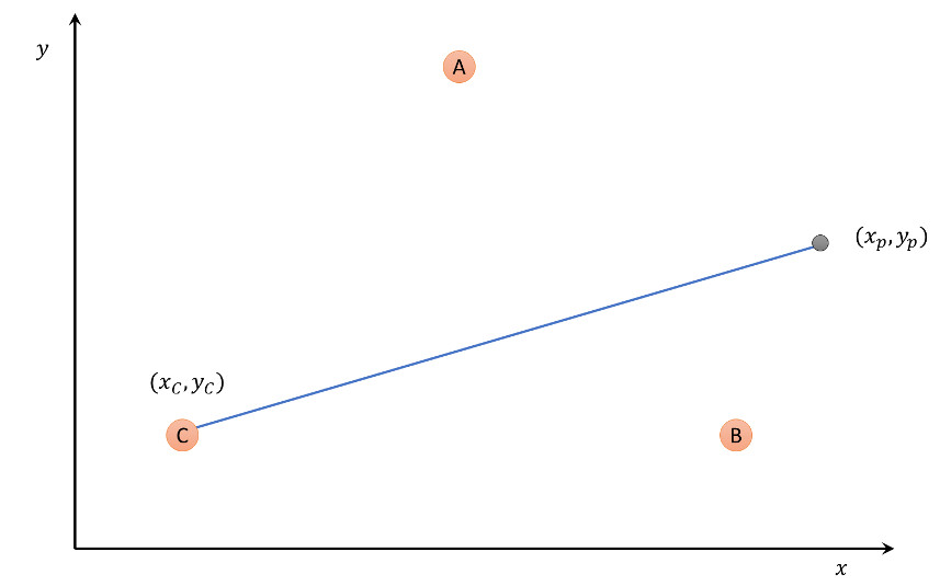
To map this procedure to a mathematical algorithm, start with the situation pictured below.

Assuming that vertex C is chosen by random, the line joining the current point to the vertex is given by

\[ \left[\begin{array}{c} x \\ y\end{array}\right] = \left[ \begin{array}{c} x_p \\ y_p \end{array} \right] + \lambda \left[\begin{array}{c} x_C – x_p \\ y_C – y_p\end{array}\right] \; , \]

where the parameter $$\lambda$$ ranges from 0 to 1, with 0 corresponding to the initial point and 1 to vertex C.  The point halfway from the initial point to the vertex C has coordinates given by substituting $\lambda = 1/2$ to yield

\[ \left[\begin{array}{c} x_{1/2} \\ y_{1/2}\end{array}\right] = \frac{1}{2}\left[ \begin{array}{c} x_p \\ y_p\end{array}\right] + \frac{1}{2} \left[\begin{array}{c} x_C \\ y_C\end{array}\right] \; . \]

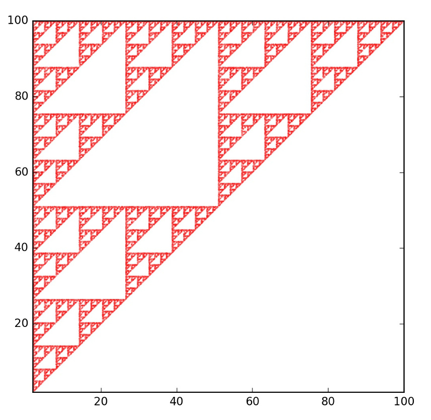
By comparing this formal transformation with the rows of the table, it is obvious that the vertices of the triangle used in the chaos game are:  A – (2,2), B – (2,100), C – (100,100).  This is nicely confirmed by putting the axes back on the figures and foregoing the aesthetic transformation used last month.

The limits of the figure are [2,100] for the x-axis and y-axis and the triangle fits perfectly into the upper left half.

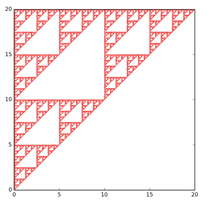
Further confirmation is obtained by changing the values of $f$ and $g$ for all three affine transformations so that the vertices are now located at: A – (0,0), B – (0,20), C – (20,20).  Rerunning the chaos game yields the following fractal

Here the limits on the plot are [0,20] for both the x- and y-axes.

With a firm understanding of what the parameters $f$ and $g$ do, next turn attention to the matrix-portion of the transformation.  Referring to the half-way point equation above, the first term on the right-hand side can be recast as

\[ \frac{1}{2} \left[ \begin{array}{c} x_p \\ y_p \end{array} \right] = \left[ \begin{array}{cc} 1/2 & 0 \\ 0 & 1/2 \end{array}\right] \left[\begin{array}{c} x_p \\ y_p\end{array} \right] \; ,\]

thus explaining what the parameters $a$, $b$, $c$, and $d$ describe.  For example, to get to point a third of the way along the line connecting the current point to the particular vertex, the table should be changed so that $a = 1/3 = d$ while keeping $b=0=c$.

Finally, the cumulative probabilities can be modified as well to create additional realizations of the game.

Next post will explore some of the various new fractals that can be obtained by fiddling with the matrix component of the affine transformation and the cumulative probabilities as a way of investigating the stability of the game to variations.

As is typical of many of the best things in life, discovery of this month’s topic involved quite a bit of serendipity.  It all started with a search for a quick reminder on how to solve a numerical set of coupled ODEs using scipy/Python and it ended with the results seen here on the chaos game.

Since it is possible that the reader is unfamiliar with this term (as was the author), a quick introduction is warranted.  In short, the chaos game is a random method for producing a deterministic fractal shape.  Its operation is in sharp contrast to the more traditional way of drawing a fractal deterministically by hand in that the chaos game teases out the fractal’s attractor by iteratively applying a set of affine transformations, each chosen randomly, to a series of points starting with a randomly chosen initial point.

Mathematically, the chaos game falls under the broader heading of an Iterated Function System (IFS) where the ith point in the plane $q_i$ is given by

\[ q_i = M^{(p)} q_{i-1} + f^{(p)} \; \]

or, in terms of arrays

\[ \left[ \begin{array}{c} x_i \\ y_i \end{array} \right] = \left[ \begin{array}{cc} a^{(p)} & b^{(p)} \\ c^{(p)} & d^{(p)} \end{array} \right] \left[ \begin{array}{c} x_{i-1} \\ y_{i-1} \end{array} \right] + \left[ \begin{array}{c} f^{(p)} \\ g^{(p)} \end{array} \right] \; .\]

The index $p$ is an integer to label the various affine transformations available, and is chosen at random at each step according to some pre-defined probability distribution.

Before getting to the Python code, which is easy to implement, it is instructive to compare and contrast the traditional method and the chaos game in generating the well-known Sierpinski Triangle fractal.

The traditional way to draw the Sierpinski Triangle starts with an equilateral triangle.

A similar triangle half in size (or a quarter in area) is removed from the middle of the larger triangle leaving an arrangement of three smaller triangles.

The process can then be applied to these smaller triangles yielding another stage of refinement.  This in turn results in a larger set of smaller triangles to which the process can be applied yet again.

Continuing on indefinitely gives the Sierpinski Triangle in all its glory.

However, there is a fundamental limit on how much can be drawn by hand or by computer, and the amount of work to obtain a successively more exact approximation in level of detail becomes increasingly more immense.

In the chaos game, the programing is much simpler and, due to the random nature of the system, all levels of detail are present simultaneously.  Central to the chaos game approach are the three affine transformations:

\[ T1: \left[ \begin{array}{c} x_i \\ y_i \end{array} \right] = \left[ \begin{array}{cc} 0.5 & 0 \\ 0 & 0.5 \end{array} \right] \left[ \begin{array}{c} x_{i-1} \\ y_{i-1} \end{array} \right] + \left[ \begin{array}{c} 1 \\ 1 \end{array} \right] \; ,\]

\[ T2: \left[ \begin{array}{c} x_i \\ y_i \end{array} \right] = \left[ \begin{array}{cc} 0.5 & 0 \\ 0 & 0.5 \end{array} \right] \left[ \begin{array}{c} x_{i-1} \\ y_{i-1} \end{array} \right] + \left[ \begin{array}{c} 1 \\ 50 \end{array} \right] \; , \]

and

\[ T3: \left[ \begin{array}{c} x_i \\ y_i \end{array} \right] = \left[ \begin{array}{cc} 0.5 & 0 \\ 0 & 0.5 \end{array} \right] \left[ \begin{array}{c} x_{i-1} \\ y_{i-1} \end{array} \right] + \left[ \begin{array}{c} 50 \\ 50 \end{array} \right] \; .\]

At each stage of the iteration, one of these transformations is selected with probability 1/3; that is to say that each is equally likely to be selected.

Four basic pieces of code are used in the implementation.

The first is a table that encodes the selection probability and the parameters for each affine transformation used in the game (i.e., each row of the table encodes the likelihood and the numbers associated with $T1$, $T2$, and so on).  The table encoding for the Sierpinski Triangle is:

sierpinski_triangle = np.array([[0.33,0.5,0,0,0.5, 1, 1],
                                [0.66,0.5,0,0,0.5, 1,50],
                                [1.00,0.5,0,0,0.5,50,50]])

Second is the Transform iteration function that takes as input the current point, the table describing the game, and a random number simulating the probability at each step.

def Transform(point,table,r):
    x0 = point[0]
    y0 = point[1]

    for i in range(len(table)):
        if r <= table[i,0]:
            N = i
            break

    x = table[N,1]*x0 + table[N,2]*y0 + table[N,5]
    y = table[N,3]*x0 + table[N,4]*y0 + table[N,6]

    return np.array([x,y])

Third is looping code that carries out the chaos game through successive applications.  The code, which, for convenience, wasn’t encapsulated in a function, looks like

N     = 100000
shape = np.zeros((N,2))
probs = np.random.random(N)
game  = sierpinski_triangle

for i in range(1,N):
    shape[i,:] = Transform(shape[i-1,:],game,probs[i])

The parameter N sets the number of desired iterations; the numpy array shape pre-allocates the space for the resulting points from the iterations and initializes the starting point to the origin.  The probabilities are also precomputed since a call to the numpy (np) random is more quickly performed when in bulk than at each step.  The game object points at the particular table encoding the transformations, here the sierpinski_triangle table defined above.  The for loop could be done faster using a list comprehension but at the loss of clarity.  Since N = 100000 takes less than a second of computation there wasn’t a compelling reason to lose the clarity.

The final step is a plot of the results.  The code that performs this is given by

start = 0

fig_shape = plt.figure(figsize=(6,6))
ax_shape  = fig_shape.add_subplot(1,1,1)
ax_shape.scatter(shape[start:,0],shape[start:,1],marker='.',color='k',s=0.01)
ax_shape.axes.set_frame_on(False)
ax_shape.xaxis.set_visible(False)
ax_shape.yaxis.set_visible(False)

The parameter start sets the number of initial points to ignore.  This is sometimes useful to suppress the initial stray n points until the game converges to the fractal attractor.

All of these pieces were put together in a Jupyter notebook.  The resulting image is

Note that the Sierpinski Triangle is rotated 45 degrees from the more usual ‘artistic’ expression.  That minor issue is easily rectified using a simple rotation matrix

c45 = 1.0/np.sqrt(2.0)
s45 = 1.0/np.sqrt(2.0)
A   = np.array([[c45,s45],[-s45,c45]])

new_shape = np.array([A.dot(shape[i,:]) for i in range(len(shape))])

where the parameters c45 and s45 are shorthand for $\cos(45 {}^{\circ}) = 1/\sqrt{2}$ and $\sin(45 {}^{\circ}) = 1/\sqrt{2}$, respectively.

The resulting image is now more aesthetically pleasing.

Making it an equilateral triangle is left as an exercise for the reader.

Note that I’ve played with the color scheme freely and inconsistently from image to image.  Picking and playing with colors is one of the most fun things about exploring the chaos game.

Future columns will look more closely at the chaos game, why it works the way it does and some of the beautiful images that can be produced.

Building on the spirit of whimsy that has been lurking in these columns of late, I thought I would devote one last post to the ambiguities and philosophical twists in natural language.  Not only do these curiosities shed light on the nature of human thought and speech, they also set a standard for any candidate trying to pass the Turing test.  After all, a human response to certain phrases should sometimes be blank confusion or a dumbfounded response like “Sorry, but I don’t have a clue what you mean.”  Other times, subtlety, irony, or humor – all decidedly human expressions – should result when a nuance in language, pointing to an elusive connection, a peculiarity of ideas, or an absurd notion present in a phrase we all take for granted, comes to the front.

The linguistic hedge will be our starting point.  The concept of a linguistic hedge (caution: this Wikipedia link, while containing some useful examples, is full of modern mangling of the language such as using “they” instead of “he” and using passive instead of active voice) is a commonplace and useful component of language that we all use, even if the phrase is unfamiliar.  Suppose you pose the question, “How hungry are you?” to a friend, and his response is, “Very hungry!”; you know that he wants some food fairly badly.  The word “very” is one of the most basic hedges and fuzzy logic often employees it as a mathematical modifier to set membership (maybe more on this in a later post).

People use hedging in a variety of ways, to emphasize degree (as in “very hungry”, or “very, very hungry”), to dodge the truth (as in “to the best of my knowledge”), and to be sarcastic (“she is very good”).  But few uses are as amusing as the use of the word “pretty.”

Ordinarily, English speakers use “pretty” as an adjective, with the typical practice being exemplified by sentences such as “She looks pretty,” or “She looks very pretty.”  However, it is fairly common, in more slang-oriented speech, to say something like “John asked, ‘How big was the rock that you hit with your car?’  Steve answered ‘It was pretty big.’”

Google’s dictionary defines pretty (adverb) as:

Just how does “pretty” turn into a linguistic hedge is a mystery (at least to me) but its use can lead to some very awkward and very funny constructions.  One construction, filled with cleverness and mirth, is the use of pretty to modify words that common speech would normally consider antithetical to the adjectival use of pretty.

For example, there is a comic book published by Image comics called Pretty Deadly.  The book centers on Jenny, the daughter of the embodiment of Death, who is both beautiful and a nearly unstoppable assassin.

An artificial intelligence capable of human-like responses would have to appreciate and, perhaps savor, the double meaning contained in the title, to allow itself to move back and forth between the two separate meanings, to imagine and possibly construct new associations inspired by the juxtaposition of two otherwise dissimilar words.

Likewise, to match its biological counterparts, it would have to enjoy the most humorous use of pretty when it modifies adjectives that are exactly opposite to its adjectival form, such as hideous, grotesque, repulsive, and so on.   Consider the following set of man’s best friends

and the fully natural way in which they are labeled.   Imagine an artificial intelligence trying to properly understand why “pretty ugly” or “pretty repulsive” is linguistically intelligible but why “pretty pretty” is just plain wrong.  Of course, one can always program the AI to work around “pretty pretty” as a corner case but take a moment to reflect on who programmed us to recognize just how bad it sounds.  Your answer should have been no one, because we just innately recognize just how stupid that phrase is.

Somehow, a true AI would need to learn and know and imagine how to use linguistic hedges to sound clever or funny or poetic without some vast if-then-else loop or training on large amounts of data that someone else blessed as proper speech.  It should know when to honor the rules and when to break them and when to invent new ones.  But such an AI is nowhere to be seen on the horizon, and that’s pretty sad.

An earlier post (Language and Thought) reflected on the question as if language effects the way we think and if so by how much.  The general conclusion is that the hypothesis that a native speaker can only think thoughts for which his mother tongue possesses a word (the so-called Sapir-Whorf thesis) is unsupported by either common sense or by empirical evidence.  However, there are numerous examples of language shaping the habits and attitudes of its native speakers in interesting and, sometimes, surprising ways.  Attitudes, being what they are, range over the entire gamut of human emotions and the emotional foci for this discussion will be humor and whimsey.

Nothing seems to separate the lower animals from humans as much as the abstract sense of humor.  While mankind shares a sense of pleasure and mirth with more primitive animals no other species exhibits humor in a spoken language littered with abstract concepts, double entendre, and shades of meaning.  A man and a dog may both laugh at someone slipping on a banana peel but only the man will find a ‘man bites dog’ joke funny (although if he does he still qualify as human?).  And if machines will ever get to the point where they can mimic man then they better learn to tell a good joke or, at least, laugh at one.

Topping the list of mirthful, silly constructions, is the buffalo grammar.  For those unfamiliar, a short summary is in order.  The word buffalo can be used as a noun (i.e. the large herd animal also known as a bison), an adjective (as in the city of Buffalo), and as a verb (meaning to fool, puzzle, baffle of mystify).  This flexibility allows English speakers to create all sorts of sentences consisting solely of that one word.

Some examples will help to illustrate.  (Note that a given sentence may have multiple meanings only one of which is used in the illustration.)

1 word:

2 words:

3 words:

4 words:

5 words:

The following youtube video gives more background (although they use another definition for buffalo as a verb – to intimidate or bully).

Far funnier is the video by Cleardino that maps a 8-buffalo-long sentence eventually into Japanese dogs in Tokyo doing unspeakable things to each other.

At the heart of all the mischief caused by all these bison is the concept of lexical ambiguity in which words with multiple senses or meanings can produce sentences and similar structures that are just flat out funny (and confusing).

In 2006, author Lynne Truss provided another wonderfully colorful and beautifully ambiguous string to add to one’s lexicon:  Eats Shoots & Leaves.  The subtitle of the work The Zero Tolerance Approach to Punctuation reveals that her true purpose is to guard society against ‘plummeting punctuation standards’ but for this work we will concentrate on the pandas (giant pandas actually) that gracefully adorn her cover – or at least as gracefully as pandas can do anything.

Depending on the punctuation, specifically the placement of commas, and context different meanings can be wrung from those three innocent words.

For example, suppose the panda in question is currently incarcerated in what animal rights activists may characterize as a gulag-for-lower-life-forms but which you and I may end up calling a zoo.  Faced with the problem of panda nutrition when may be inclined to bring our black-and-white inmates eats, shoots, and leaves meaning food from the local pub (eats), bamboo shoots, and the leaves from a particular nice tree over on the west side of the cage.

Further suppose that an expert on mammalian physiology with a specialty in primates and having world-class expertise in pandas comes by while we are trying to feed one of our bouncing bears potato chips.  He may disgustingly shake his head and yell ‘eats shoots and leaves’ meaning ‘that bear consumes plant shoots and tree leaves’.

Furthermore, suppose that our panda, now aware of our shabby treatment, pulls a loaded revolver (but from where) and ends our miserable existence.  At the inquest, there may be a witness who describes what he saw, in present tense so as to increase the vividness of his description, by saying:

meaning that the panda ate a bite, pulled a gun and shot us, and then skedaddled back to China since there are no extradition agreements that will bring him to justice in the US.

Clearly Truss intends us to take punctuation so seriously that she is willing to use humor to drive her points home.

And lest the reader thinks that this kind of fun is confined only to English consider the following very old and venerated poem in Chinese.

This kind fun (and confusion) makes natural language a real challenge for machine intelligence.  For now, systems are barely able to translate language constructions intended to be clear and communicative.  So it seems a safe bet to say that AI has a long way to go before it is impishly playing with the language.  But when it does, that’s when we should start worrying or maybe laughing, I just don’t know.

It is an often-stated and, I think, well-established idea in the physical sciences that the ‘mathematical words’ used to express an idea are often as important as—or, in certain circumstances, more important than—the ideas being expressed.  ‘Notation matters’ is the catchphrase, and it reflects the belief that better ways of encapsulating an idea lead to better ideas (see e.g. S.S. Chern’s Differential Geometry; Its Past and Its Future).  Basically, the mathematical words used either enable or limit the thoughts that can be conceived or expressed.

The poster child for this belief is the emergence of vector calculus as the language used in field theories.  The physical idea that no magnetic monopoles exist in nature is much harder to see in component form

\[ \frac{\partial B_x}{\partial x} + \frac{\partial B_y}{\partial y} + \frac{\partial B_z}{\partial z} = 0 \]

than in the more compact

\[ \vec \nabla \cdot \vec B = 0 \; .\]

The same argument seems to be widely held in computing.  Certain programming languages (LISP or one of its dialects) are often said to shape how a programmer actually thinks about programming.  Proponents of object-oriented or functional programming maintain that it is easier to express algorithms in these paradigms because they allow the programmer to abstract more complex ideas, thus being able to focus on the logic without being bogged down in the day-to-day syntax.

These ideas have plenty of anecdotes supporting them (and, perhaps, some scientifically gathered and analyzed data) and it is natural to wonder if the same holds true for natural languages; does one’s mother tongue limit the thoughts that one can think?

The simple answer is no.  The mathematical experience teaches us that new ideas can be expressed with the old words, but the result is that we often do so by adding new words to encapsulate these ideas.  In terms of the example above, the compact expression $\vec \nabla \cdot \vec B$ allows one to think more broadly about the magnetic field in the abstract, but the ‘clunky’ coordinate expression is what one uses when one wants to actually compute something.

Nonetheless, philosophers and linguists are not inclined to trust experiences from mathematicians and scientists, and they’ve looked into this point on their own.  After all, the traditional overlap between thought and speech traces its origin back to the ancient philosophers, who regarded the ability to speak as a hallmark indicating that man is a rational animal.  However, the modern renaissance seems to date from 1940 with the work of Benjamin Lee Whorf.

In his article Does Your Language Shape How You Think?, Guy Deutshcer of the New York Times discusses Whorf’s 1940 article entitled Science and Linguistics, which claimed that language imposes a different form of reality on one set of speakers versus another.  As Deutshcer relates, Whorf asserted that, if a language didn’t have a word for a concept, the concept would be unknown to speakers of this language.  It is hard to believe that this assertion was really what Whorf believed or, if so, that it was taken seriously, as there is a reductio ad absurdum argument that would deduce that sentences with multiple words used to express complex ideas would never be needed or used, except to make new words.

Nevertheless, Deutshcer provides some interesting ‘refutations’ of the Sapir-Whorf thesis (Edward Sapir was Whorf’s teacher).  For example, some languages, like Chinese, don’t have a formally delineated future tense whereas English does.  And yet the two sentences “Are you coming tomorrow?” (more Chinese-like) and “Will you come tomorrow?” (less Chinese-like) are equivalent, suggesting that considerations about the future for a native Chinese speaker are not different from those whose native tongue is English, even if they express themselves differently.  Likewise, English didn’t have a single word equivalent for schadenfreude, but English-speakers still indulged in that behavior, and that word has essentially been incorporated into English.

Despite the fact that Whorf’s main conclusions seem to have been wrong, the notion that language shapes thoughts in addition to thoughts shaping language does seem to have some truth.  Deutscher quotes the linguist Roman Jakobson as saying that “languages differ essentially in what they must convey and not in what they may convey”.  To get a sense of what that means, he presents the sentence “I spent yesterday with a neighbor.”, which in English leaves the sex of the neighbor entirely unspecified whereas German, French, or Spanish require the speaker to specify a gender.

Joshua Hartshorne, writing for Scientific American, explores some other aspects in his article Does Language Shape What We Think?  He presents the interesting case of the Pirahã, who have no precise counting words, just general notions.  When asked to exchange, say, seventeen rocks for an equivalent number of sticks, the Pirahã can match the objects one-to-one but they can’t count out seventeen sticks abstractly to prepare the exchange in advance.  Does this behavior suggest that, since they don’t have a word for the abstract idea of seventeen, they don’t know what seventeen is?  Hartshorne doesn’t think so—neither do I.  They just don’t have any abstraction for the counting process.  This is a common problem that English speakers encounter for incredibly large numbers.  I don’t know what a trillion dollars looks like or can buy but I do know how to abstractly denote it in symbols.

In her article Does Language Affect Thought?, Karen Lewis also explores the Sapir-Whorf thesis.  The primary example she discusses centers around mass nouns.  Mass nouns are nouns like mass, water, snow, meat, beer versus count nouns such as chair, pencil, one fish, two fish, red fish, blue fish.  According to Lewis, Whorf maintained that the Hopi had no mass nouns and so they perceived the world differently than we do.  She cites several experiments that suggest that, while the presence or absence of mass nouns in a language influences how the world is linguistically categorized, there is no evidence that the language influences how the speaker conceptualizes the world.

That said, it is clear that language shapes the attitudes, emotions, and preconceptions of its speakers.  In languages with gendered nouns, the adjectives used to describe these nouns depend on the gender of the noun.

What can we conclude from all these examples (and the others found in the articles cited above)?  I think the safest thing to say is that the language we speak doesn’t inhibit us from thinking new thoughts for which we don’t have pre-existing words.  But it can shape how we feel, how quickly we process thoughts, and how we express ourselves.  In a nutshell, underneath we are all the same even if we express ourselves quite differently.

Two earlier posts (An A* Drama and A Cross-Country A*) introduced the A* algorithm, how it manages to find the shortest path (more on this below), and how it can also handle terrain costs.  This post was meant to cover a minor point that was purposely omitted until now.

Unfortunately, this post must also serve as a mea culpa in which I need to apologize for a gross error in my previous two explanations.  The error became apparent as I worked up this column for last month’s installment and the discovery of the error derailed that post in favor of the one on compression and the pigeon hole principle.

In the previous two A* posts, the explanation stated that the scoring of the spots placed on the open list consisted of two parts: 1) the terrain cost (the cost to move onto the spot) and 2) the heuristic cost (an estimate of how far the spot is from the goal).  I forgot to include the total cost from the starting space, which is the sum total of all the movement costs to get to that spot.  Tracking that cost is vital to performing the re-parenting step that takes out any ‘kinks’ in the path that result from random choices the algorithm must make when picking between two spots of equal cost.

Despite this omission, the algorithm actually performed quite well in the two cases examined and it found the shortest pay in the wayfarer example (A Cross-Country A*) where the terrain costs were the primary driver and no obstacles were present.  It fared slightly worse in the original example with the angry snake and the man who poked him (An A* Drama), finding almost the shortest path, being only one step too long.  Sadly, that error escaped my notice for some time.

Fortunately, the error came and presented itself quite clearly when I returned to the snake v. man drama to explain re-parenting.   To see what re-parenting involves consider this step in the snake’s pursuit of his vengeance.

Faced with two spaces, (7,1) and (7,2), with the same total cost of 8 – 1 for terrain (upper right) and 4 for the heuristic (lower left), for a movement cost of 5 (lower right), and a cost of 3 steps from the starting space (black square in the center) – the snake randomly chooses to explore gird space (7,2).  Doing so opens up (i.e. places on the open list) spots (7,1), (8,1), (6,2), (8,2), (6,3), (7,3), and (8,3), parents them all to (7,2), and scores them all as having a total cost from the starting space of 4, since any path to these spaces must first go through (7,2), which is 3 steps away from the starting space.

The key point to note, is that the shortest path from the starting space to spaces (6,3) and (7,3) (for a total cost from start of 3) passes through spot (6,2), which is not explored first because of its greater cost.  As a result, the current path to either (6,3) or (7,3) first goes past them to the right while it approaches from below before going back to the left as it arrives; the last three spots in the path are connected as (6,1) -> (7,2) -> (6,3).  Because of its shape, I call such a sub-optimal path a kink.

Now that we recognized the kink, what are we to do with it?  Well, for the time being we just let it alone.  When the algorithm finally explores one of these points, we simply look to see if shifting its parent from (7,2) to some other nearby space will lower the total cost from the starting spot.  If so, then the parent is changed and the algorithm continues essentially unchanged.

To be concrete, consider the situation a bit further in the snake’s search for a path to his foe.  After meandering in the lower right for a while, the snake’s exploration has carried him to space (7,3), which, as a reminder, has received a total cost from the start space of 4 and which is parented to (7,2).

As the snake explores space (7,3), he looks around to see if re-parenting the space to any of the neighboring spaces will lower the total cost from the starting space.  He notes that re-parenting (7,3) to (6,2) will lower that total cost from the starting space by 1 and he does so.  The box containing the new cost has been colored orange to reflect this change.

Because (7,4) had been opened and scored when (8,3) was explored, it also will be re-parented when the snake recognizes the strategic importance of slithering through (7,4).

The final path requires the snake to make 10 steps to reach his victim.

It is a matter of a few minutes of playing with other paths to convince oneself that this is the smallest cost to wreak his revenge.  Of course, the path passing through (6,3) -> (7,4) is equally short but won’t be found by the A* since the heuristic scoring tends to pull the paths to the right even though the ‘escape route’ requires moving to the left.  Also note, that without re-parenting, the kink would have cost an extra step, driving the total cost to 11.

So, there you have it.  A corrected and complete presentation of the A* algorithm.  Sorry for the confusion, but, at least, the error helped to frame the importance of re-parenting in finding the shortest path.