
This month’s installment will be the final column of this series on the chaos game. As befitting any swan song, this ending should be artistic and dramatic and awe-inspiring. Unfortunately, the chaos game isn’t really dramatic or awe-inspiring – at least for most people – but it can be quite artistic. The patterns that can be produced can be quite beautiful and pleasing to the eye. So, this article will be mostly a tour of our local digital museum displaying the various works of art that one can produce using either the code heretofore presented or with some minor modifications.
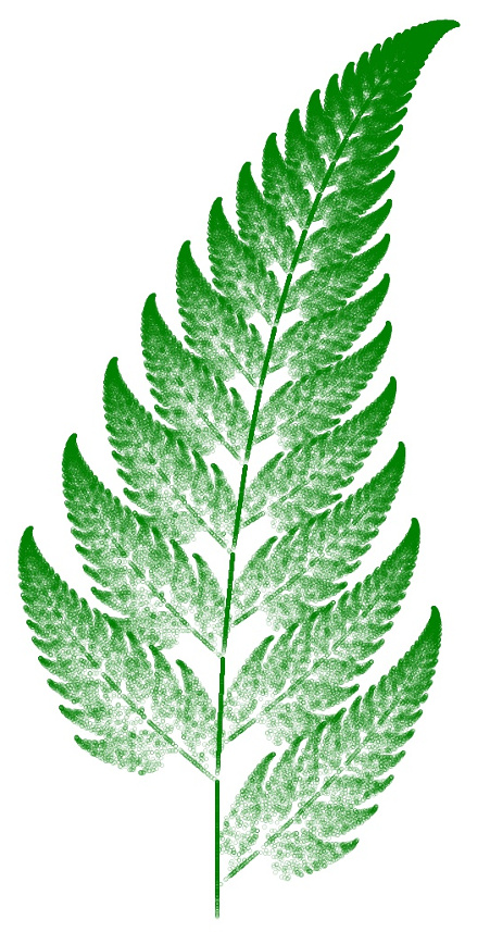
The first entry in our tour is the Barnsley fern, which is a self-similar structure invented by Michael Barnsley to resemble the black spleenwort fern. There are four entries into the set affine mappings that comprise the game:
barnsley_fern = np.array([[0.01,   0,      0,    0,0.16,0,   0],
                          [0.86, 0.85,  0.04,-0.04,0.85,0,1.60],
                          [0.93, 0.20, -0.26, 0.23,0.22,0,1.60],
                          [1.00,-0.15,  0.28, 0.26,0.24,0,0.44]])
When run through the chaos game, a remarkably pleasing fern frond is found (alliteration, a sure sign of class).
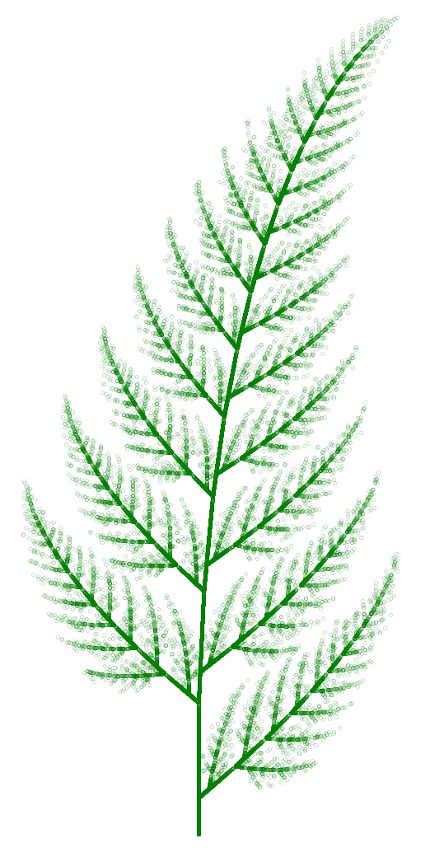
Surprisingly, one of the affine mappings in the table has only a 1 percent chance of being selected. Modification of the first entry in the table of affine mappings from 0.01 to 0.2,
barnsley_fern_2 = np.array([[0.20,   0,      0,    0,0.16,0,   0],
                            [0.86, 0.85,  0.04,-0.04,0.85,0,1.60],
                            [0.93, 0.20, -0.26, 0.23,0.22,0,1.60],
                            [1.00,-0.15,  0.28, 0.26,0.24,0,0.44]])
thus increasing the probability of using the first mapping at the expense of the second, results in a slightly less luxurious, or mangier but, nonetheless, quite similar frond.
This result strongly supports the conclusion from the last post that the chaos game operations on this set of affine maps seems to be quite stable against changes. Play of this kind also opens the door to the idea of a meta chaos game where the exact set of affine maps used at any iteration is either subjected to small random variations or is picked from a larger set. In the latter case, one can imagine a meta algorithm selecting between the barnsley_fern and barnsley_fern_2 tables for each frond as part of a larger plant or switching between the two at random. Perhaps this type of numerical experiment will form the subject of a future column.
But now back to the tour.
Other mathematicians, professional and amateur alike, have played with the set of affine mappings to create similar plant-like results. An interesting example, called here the Flatter Fern, has as its set of affine mappings
flatter_fern = np.array([[0.02,0,0,0,0.25,0,-0.4],
                         [0.86,0.95,0.005,-0.005,0.93,-0.002,0.5],
                         [0.93,0.035,-0.2,0.16,0.04,-0.09,0.02],
                         [1.00,-0.04,0.2,0.16,0.04,0.083,0.12]])
Using this table in the chaos game gives
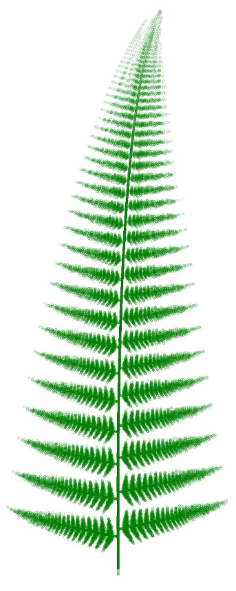
As in the previous case, the structure is self-similar but each of the leaf groups is thinner and straighter than in the Barnsley fern.
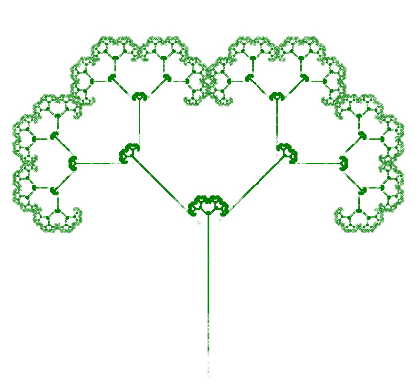
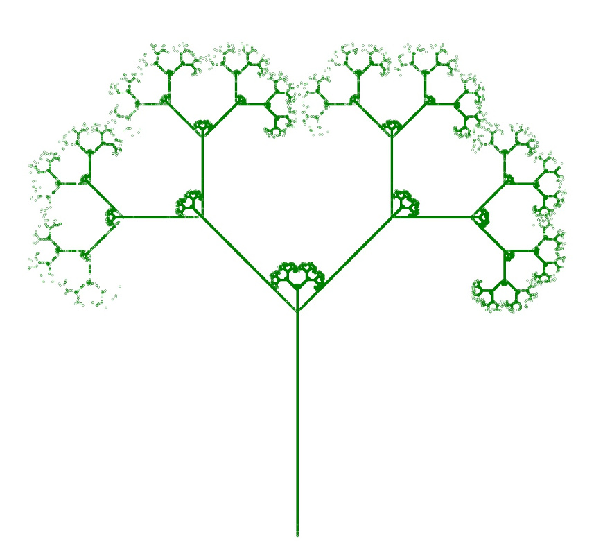
Keeping with the botanical theme, another fan favorite is the Fractal Tree. Its set of affine maps is
fractal_tree  = np.array([[0.05,   0,    0,    0, 0.5, 0,  0],
                          [0.45,0.42,-0.42, 0.42,0.42, 0,0.2],
                          [0.85,0.42, 0.42,-0.42,0.42, 0,0.2],
                          [1.00, 0.1,    0,    0, 0.1, 0,0.2]])
Running the chaos game with this table gives something that looks more like broccoli than it does a tree.
Once again, one can play with the stability of the game by adjusting the relative probabilities. By upping the probability of the first map of the set from 0.05 to 0.25, giving the following table
fractal_puff  = np.array([[0.25,   0,    0,    0, 0.5, 0,  0],
 [0.45,0.42,-0.42, 0.42,0.42, 0,0.2],

[0.85,0.42, 0.42,-0.42,0.42, 0,0.2],

[1.00, 0.1,    0,    0, 0.1, 0,0.2]])
the chaos game produces a Fractal Puff
which suggests that the outer edge is soft, fuzzy, and worn away.
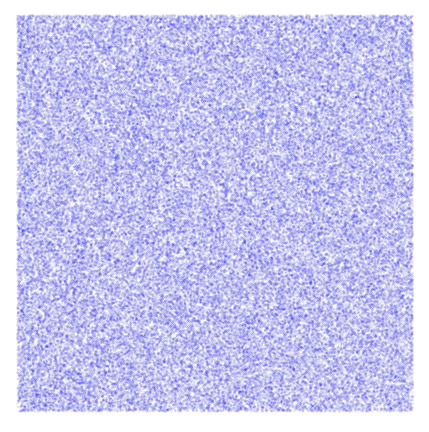
In the next wing of the museum awaits a curious set of geometric shapes. The one we will examine in detail is the Square, whose set of affine maps is displayed in the following table.
square  = np.array([[0.25,0.5,0,0,0.5, 1, 1],
                    [0.50,0.5,0,0,0.5,50, 1],
                    [0.75,0.5,0,0,0.5, 1,50],
                    [1.00,0.5,0,0,0.5,50,50]])
In this case, running the chaos game with this table results in a uniformly filled region.
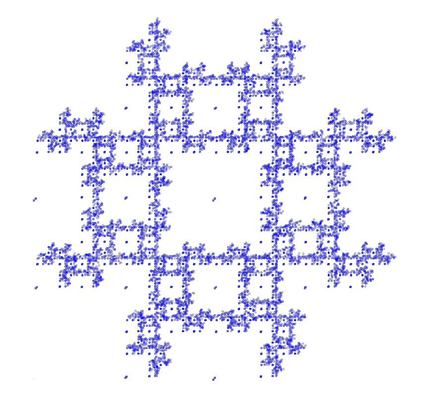
The trick to making a fractal appear is to restrict the selection of the vertex so that the same vertex cannot be picked in a row. The easiest modification to the code used in these explorations is to create a new transformation function
def Transform2(point,table,r,prev_N):
    x0 = point[0]
    y0 = point[1]
    for i in range(len(table)):
        if r <= table[i,0]:
            N = i
            break
    if N != prev_N:
        x = table[N,1]*x0 + table[N,2]*y0 + table[N,5]
        y = table[N,3]*x0 + table[N,4]*y0 + table[N,6]
    else:
        x = np.NaN
        y = np.NaN

    return np.array([x,y]), N
that is aware of the previous vertex (the variable prev_N) and returns a null result for the new point. Testing the return value keeps the ‘bad’ point out of the results giving the following pattern
The Wikipedia article on the chaos game, has a stunning gallery of geometric shapes that result from by similar types of rules restricting vertices. Particularly interesting are the pentagon examples by Edward Haas.
The first one, shows the resulting pattern by using an analogous set of maps to the square and restricting the vertex to be strictly different from the one before.
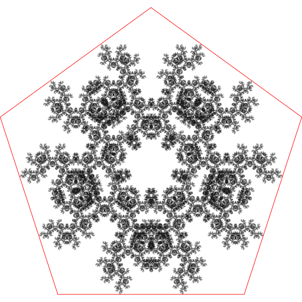
In Haas’s second case, the pattern results from using the same table as his first case, but with the restriction that the new vertex cannot be 1 or 4 places away from the two previously chosen vertices.
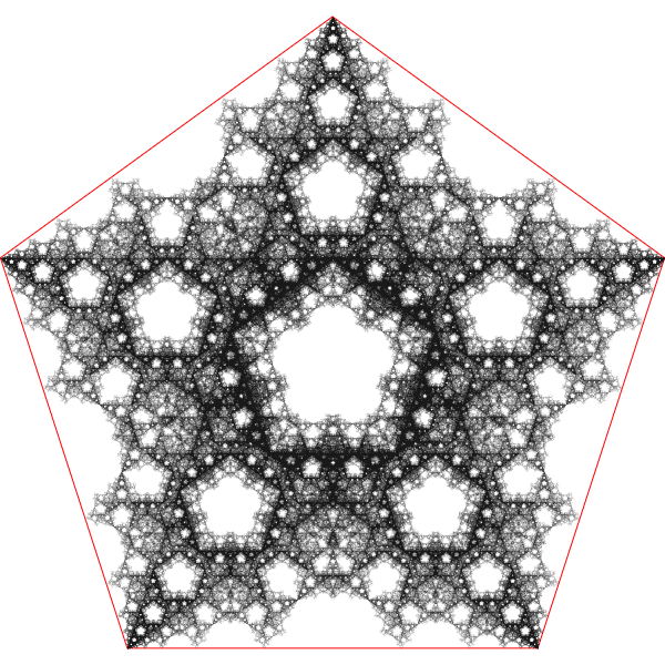
While both cases exhibit five-fold symmetry the differences that arise solely due to the restriction on the allowed vertices is startling.
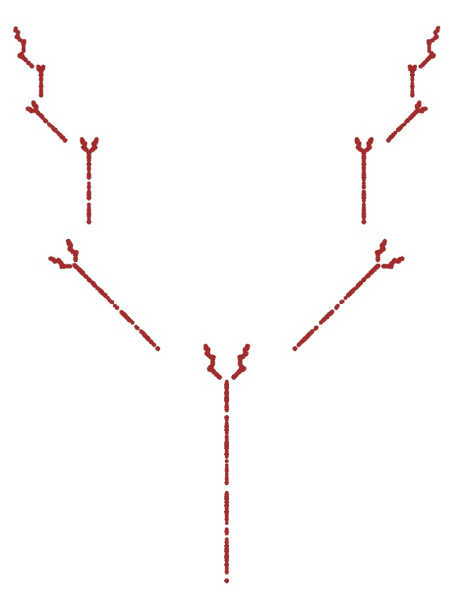
The final exhibit is a mix of the botanical and the geometric. The Fractal Tree table was used with the vertex restriction rule used with the square. The resulting Fractal Twig is beautiful in its brutal desolation (always wanted to talk like a snooty, pretentious modern art dealer)
So, it seems as if the sky is the limit in creating digital art using the chaos game. I suspect we’ve only scratched the surface.