Now having introduced the chaos game and analyzed how a single iteration works, it is worth taking stock of what we actually know.  Clearly the repeated application of the affine map causes points to collect only in certain places in the plane creating the self-similar fractals that are often called the attractors of the map or strange attractors.  We’ve also established what the parameters of the affine map do in the particular case of the Sierpinski triangle, getting a sense of how those parameters map to the rules discussed in the Numberphile video.  But the exact mechanism for why only certain points are hit is based on some specialized mathematics and little intuition is obtained from pursuing the study without a lot of initial effort being devoted to understanding the ‘nuts and bolts’.

So, this post is devoted to an experimental approach to the chaos game that produces the Sierpinski triangle.  Each experiment performed involves changing one or more of the parameters that make up the affine maps used in the game and then observing what happens to the pattern produced.  Doing so will help us understand the stability of the map.

Stability can be defined in numerous ways.  There are definite schools of thought with different interpretations.  For this exploration of the chaos game, I will define two types of stability:  deterministic and stochastic.

Deterministic stability looks to see in what range of parameters does the chaos game yield fractal-like results.  The parameters themselves are chosen at the beginning of the game and remain fixed during its progression.   The idea is to answer such questions as:  How accurate do the parameters need to be?  How many different shapes or patterns result?  How many different types of games are there?

To get a sense of what answers may result and to clarify what is meant by ‘types of games’, consider the investigation detailed in the last post.  As a direct byproduct of understanding a single iteration, the significance of the constant terms $f^{(p)}$ and $g^{(p)}$ used in three Sierpinski affine maps became clear; multiplying these parameters by two gave the coordinates of vertices of the triangle.  The same Sierpinski triangle resulted even if these values were changed.  Thus, the family of all possible values for $f^{(p)}$ and $g^{(p)}$ form an equivalence class where the scale and overall geometry may change but the shape is undeniably a Sierpinski triangle.  I term this equivalence class as a single game.

In contrast, stochastic stability involves regarding the parameters of the affine maps as random variables, which vary at each iteration.  The time history of each random variable forms a unique realization that is different each time the game is played.  This aspect can be quite important because noise can creep into the game in a variety of scenarios.  Computationally, the finite precision floating point representation of the rational numbers in the game are not exact and small errors arise as the game progresses through its iterations.  Physically, an analog of the game in the material world is a messy affair with the parameters of the maps only inexactly realized due to all the small but unmodelled effects.

One possible way of implementing a stochastic game would be to generalize the deterministic expression for a new point $(x,y)$ in the Sierpinski triangle game,

\[ \left[ \begin{array}{c} x \\ y \end{array} \right] = \left[ \begin{array}{cc} 1/2 & 0 \\ 0 & 1/2 \end{array} \right] \left[ \begin{array}{c} x_{current} \\ y_{current} \end{array} \right] + \frac{1}{2} \left[ \begin{array}{c} x_{vertex} \\ y_{vertex} \end{array} \right] \; , \]

(where $(x_{vertex},y_{vertex})$ are the coordinates of one of the three vertices of the triangle, chosen randomly, and $(x_{current},y_{current})$ is the current points coordinates) to a physical system by making the transformation matrix look like

\[ \left[ \begin{array}{cc} 1/2 & 0 \\ 0 & 1/2 \end{array} \right] \rightarrow \left[ \begin{array}{cc} 1/2 + \eta_{11} & \eta_{12} \\ \eta_{21} & 1/2 + \eta_22 \end{array} \right] \; , \]

where the $\eta_{ij}$ are random variables, with some specified moments, reflecting noise that is ubiquitous in the world.

For this post, we’ll content ourselves with exploring deterministic stability for the Sierpinski triangle, looking at what results from changing the values in the transformation matrix and the relative probabilities that each vertex is selected.  In order to facilitate the experiments, each game’s results will be over-plotted (in black) the results from the standard Sierpinski triangle (red).

The first experiment, we’ll change the transformation matrix so that the new point is only moved one third along the line from the current point to the vertex (this was actually suggested in the Numberphile video).  This modification amounts to the following change for the transformation matrix

\[ \left[ \begin{array}{cc} 1/2 & 0 \\ 0 & 1/2 \end{array} \right] \rightarrow \left[ \begin{array}{cc} 1/3 & 0 \\ 0 & 1/3 \end{array} \right] \; . \]

Running the game gives

At first glance, lowering the values in the transformation matrix seems to have simply shrank the scale of the triangle but closer inspection shows that there is a fundamental change in the geometry.  The missing ‘center piece’ is now a squat hexagon instead of a triangle as is more easily seen with the following annotated figure.

This small change has resulted in a new, but closely related game.

Scaling up the values in the transformation matrix from $1/2$ to $3/4$ leads to no discernible structure (with the original triangle now peaking thru in the lower left corner).

This result looks as if scaling the values in the transformation matrix above $1/2$ causes the points to overlap, suggesting that the value of $1/2$ is some sort of divider or separatrix between non-overlapping and overlapping points.  We might expect that a small value above one half, say $0.55$ would begin to blur the Sierpinski triangle by creating a small amount of overlap.  Running the game with this value yields

Some of the overlap regions are highlighted within red circles and the remaining ones can deduced by the symmetry exhibited by this self-similar fractal.

Likewise, a value of $0.45$ produces a triangle where the sub-triangles no longer smoothly join together but where there are gaps.

If this process were to occur in a physical system (and there are certain researchers constructing such systems – see Physicists wrangled electrons into a quantum fractal) then the scales selected in the transformation matrix must stay confined to a relatively narrow range of parameter space ($0.45-0.55$) before the results become so different as to suggest that the system is fundamentally different.  That said, the geometry produced by the game, regarded strictly in a visual sense, is remarkably resilient.  Triangles within triangles result over a fairly wide range of values.

The results of the final experiment show that the game is even much more tolerant to changes in the probabilities that determine how often each vertex is picked.  In the original implementation of the game, each vertex had a $1/3$ chance of being the one selected.  To see how sensitive the game is to changes in this respect, the relative probabilities were adjusted so that one vertex had an 80% chance of being selected while there was only a 10% chance of selecting from the remaining two.  As the figure below shows, the result of this change are to simply ‘ghost out’ the vertices that are less likely.

The conclusion here is straightforward.  The chaos game method of producing the Sierpinski triangle is remarkably stable to a range of deterministic changes in the parameter set.  This robustness makes the chaos game a convenient numerical laboratory for exploring other emergent fractals, some of which we will see in the next post.

Last month’s blog introduced the idea of the chaos game, which is a simple and compact computing method for generating deterministic fractals using a Monte Carlo-like random method.  The central ingredients of the chaos game are an affine transformation of the plane

\[ \left[ \begin{array}{c} x_i \\ y_i \end{array} \right] = \left[ \begin{array}{cc} a^{(p)} & b^{(p)} \\ c^{(p)} & d^{(p)} \end{array} \right] \left[ \begin{array}{c} x_{i-1} \\ y_{i-1} \end{array} \right] + \left[ \begin{array}{c} f^{(p)} \\ g^{(p)} \end{array} \right] \; , \]

which expresses the current point (labeled by the index i) in terms of the previous point (labeled by the index i-1) in terms of known, fixed parameters $\{a^{(p)}, b^{(p)}, c^{(p)}, d^{(p)}, f^{(p)}, g^{(p)}\}$.  The index $p$ is an integer label for the various affine transformations available and is chosen at random at each step, according to some pre-defined probability distribution.  For the Sierpinski triangle discussed in the previous post, $p$ can take on the values (1,2,3) each with probability 1/3.

It is convenient to package all the information into a table with each row corresponding to a one of the affine transformations.  For the Sierpinski triangle, the table is given by

, which is directly translated into the numpy array

sierpinski_triangle = np.array([[0.33,0.5,0,0,0.5, 1, 1],
                                [0.66,0.5,0,0,0.5, 1,50],
                                [1.00,0.5,0,0,0.5,50,50]])

used for simulation (details in the previous post).

The above material, which is a quick recap of last month’s entry, sets the stage for this post, which focuses on understanding how the structures emerge from such a simple set of rules.

A good starting point for that understanding is the Numberphile video on the chaos game

The presenter, a mathematician by the name of Ben Sparks, starts by showing how the chaos game for the Sierpinski triangle is played by examining single iterations performed by hand.   He performs a single iteration by taking the initial point, rolling a six-sided die (yes die is the correct word for the singular – like Sparks that grammatical rule confuses me as well) to randomly pick one of the three vertices, connecting the point to the chosen vertex with a straight line, and then establishing the new point at a distance halfway along that line.

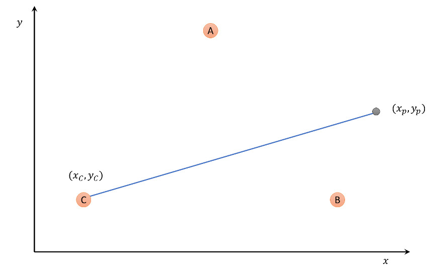
To map this procedure to a mathematical algorithm, start with the situation pictured below.

Assuming that vertex C is chosen by random, the line joining the current point to the vertex is given by

\[ \left[\begin{array}{c} x \\ y\end{array}\right] = \left[ \begin{array}{c} x_p \\ y_p \end{array} \right] + \lambda \left[\begin{array}{c} x_C – x_p \\ y_C – y_p\end{array}\right] \; , \]

where the parameter $$\lambda$$ ranges from 0 to 1, with 0 corresponding to the initial point and 1 to vertex C.  The point halfway from the initial point to the vertex C has coordinates given by substituting $\lambda = 1/2$ to yield

\[ \left[\begin{array}{c} x_{1/2} \\ y_{1/2}\end{array}\right] = \frac{1}{2}\left[ \begin{array}{c} x_p \\ y_p\end{array}\right] + \frac{1}{2} \left[\begin{array}{c} x_C \\ y_C\end{array}\right] \; . \]

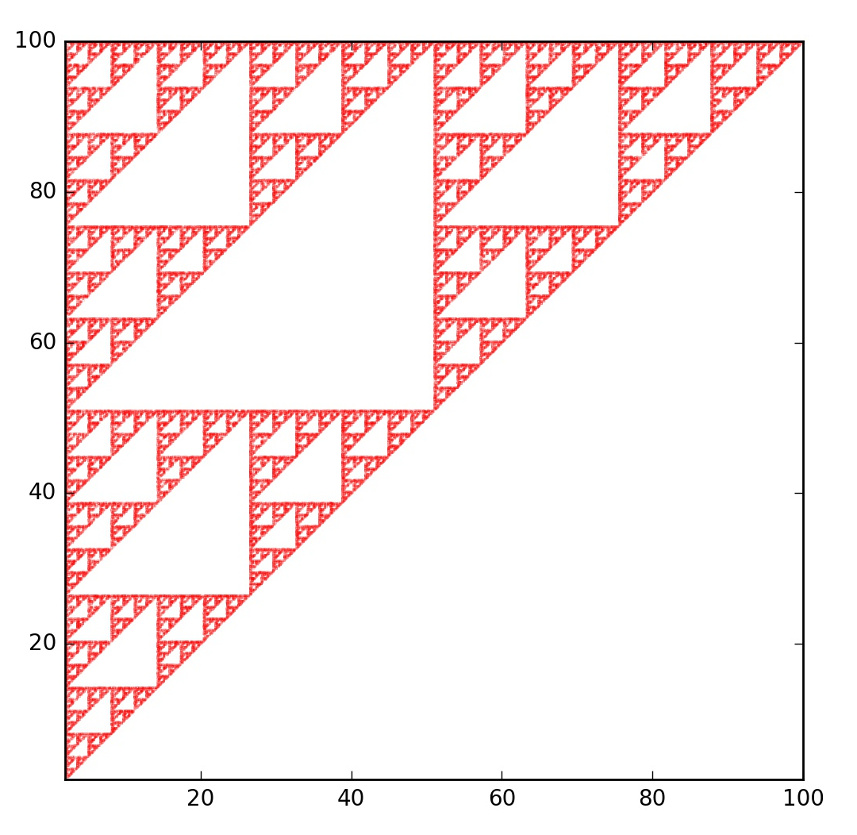
By comparing this formal transformation with the rows of the table, it is obvious that the vertices of the triangle used in the chaos game are:  A – (2,2), B – (2,100), C – (100,100).  This is nicely confirmed by putting the axes back on the figures and foregoing the aesthetic transformation used last month.

The limits of the figure are [2,100] for the x-axis and y-axis and the triangle fits perfectly into the upper left half.

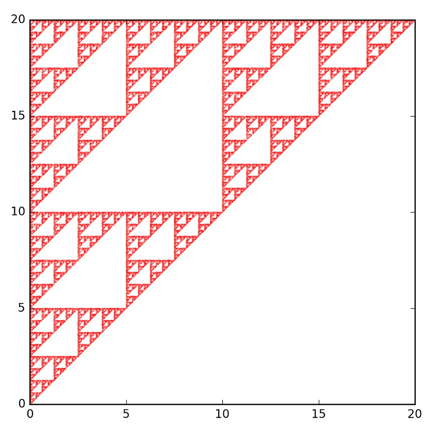
Further confirmation is obtained by changing the values of $f$ and $g$ for all three affine transformations so that the vertices are now located at: A – (0,0), B – (0,20), C – (20,20).  Rerunning the chaos game yields the following fractal

Here the limits on the plot are [0,20] for both the x- and y-axes.

With a firm understanding of what the parameters $f$ and $g$ do, next turn attention to the matrix-portion of the transformation.  Referring to the half-way point equation above, the first term on the right-hand side can be recast as

\[ \frac{1}{2} \left[ \begin{array}{c} x_p \\ y_p \end{array} \right] = \left[ \begin{array}{cc} 1/2 & 0 \\ 0 & 1/2 \end{array}\right] \left[\begin{array}{c} x_p \\ y_p\end{array} \right] \; ,\]

thus explaining what the parameters $a$, $b$, $c$, and $d$ describe.  For example, to get to point a third of the way along the line connecting the current point to the particular vertex, the table should be changed so that $a = 1/3 = d$ while keeping $b=0=c$.

Finally, the cumulative probabilities can be modified as well to create additional realizations of the game.

Next post will explore some of the various new fractals that can be obtained by fiddling with the matrix component of the affine transformation and the cumulative probabilities as a way of investigating the stability of the game to variations.

As is typical of many of the best things in life, discovery of this month’s topic involved quite a bit of serendipity.  It all started with a search for a quick reminder on how to solve a numerical set of coupled ODEs using scipy/Python and it ended with the results seen here on the chaos game.

Since it is possible that the reader is unfamiliar with this term (as was the author), a quick introduction is warranted.  In short, the chaos game is a random method for producing a deterministic fractal shape.  Its operation is in sharp contrast to the more traditional way of drawing a fractal deterministically by hand in that the chaos game teases out the fractal’s attractor by iteratively applying a set of affine transformations, each chosen randomly, to a series of points starting with a randomly chosen initial point.

Mathematically, the chaos game falls under the broader heading of an Iterated Function System (IFS) where the ith point in the plane $q_i$ is given by

\[ q_i = M^{(p)} q_{i-1} + f^{(p)} \; \]

or, in terms of arrays

\[ \left[ \begin{array}{c} x_i \\ y_i \end{array} \right] = \left[ \begin{array}{cc} a^{(p)} & b^{(p)} \\ c^{(p)} & d^{(p)} \end{array} \right] \left[ \begin{array}{c} x_{i-1} \\ y_{i-1} \end{array} \right] + \left[ \begin{array}{c} f^{(p)} \\ g^{(p)} \end{array} \right] \; .\]

The index $p$ is an integer to label the various affine transformations available, and is chosen at random at each step according to some pre-defined probability distribution.

Before getting to the Python code, which is easy to implement, it is instructive to compare and contrast the traditional method and the chaos game in generating the well-known Sierpinski Triangle fractal.

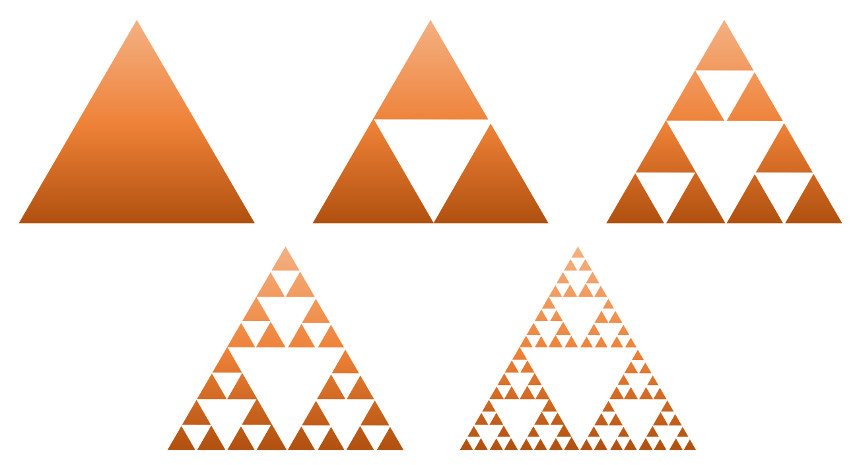
The traditional way to draw the Sierpinski Triangle starts with an equilateral triangle.

A similar triangle half in size (or a quarter in area) is removed from the middle of the larger triangle leaving an arrangement of three smaller triangles.

The process can then be applied to these smaller triangles yielding another stage of refinement.  This in turn results in a larger set of smaller triangles to which the process can be applied yet again.

Continuing on indefinitely gives the Sierpinski Triangle in all its glory.

However, there is a fundamental limit on how much can be drawn by hand or by computer, and the amount of work to obtain a successively more exact approximation in level of detail becomes increasingly more immense.

In the chaos game, the programing is much simpler and, due to the random nature of the system, all levels of detail are present simultaneously.  Central to the chaos game approach are the three affine transformations:

\[ T1: \left[ \begin{array}{c} x_i \\ y_i \end{array} \right] = \left[ \begin{array}{cc} 0.5 & 0 \\ 0 & 0.5 \end{array} \right] \left[ \begin{array}{c} x_{i-1} \\ y_{i-1} \end{array} \right] + \left[ \begin{array}{c} 1 \\ 1 \end{array} \right] \; ,\]

\[ T2: \left[ \begin{array}{c} x_i \\ y_i \end{array} \right] = \left[ \begin{array}{cc} 0.5 & 0 \\ 0 & 0.5 \end{array} \right] \left[ \begin{array}{c} x_{i-1} \\ y_{i-1} \end{array} \right] + \left[ \begin{array}{c} 1 \\ 50 \end{array} \right] \; , \]

and

\[ T3: \left[ \begin{array}{c} x_i \\ y_i \end{array} \right] = \left[ \begin{array}{cc} 0.5 & 0 \\ 0 & 0.5 \end{array} \right] \left[ \begin{array}{c} x_{i-1} \\ y_{i-1} \end{array} \right] + \left[ \begin{array}{c} 50 \\ 50 \end{array} \right] \; .\]

At each stage of the iteration, one of these transformations is selected with probability 1/3; that is to say that each is equally likely to be selected.

Four basic pieces of code are used in the implementation.

The first is a table that encodes the selection probability and the parameters for each affine transformation used in the game (i.e., each row of the table encodes the likelihood and the numbers associated with $T1$, $T2$, and so on).  The table encoding for the Sierpinski Triangle is:

sierpinski_triangle = np.array([[0.33,0.5,0,0,0.5, 1, 1],
                                [0.66,0.5,0,0,0.5, 1,50],
                                [1.00,0.5,0,0,0.5,50,50]])

Second is the Transform iteration function that takes as input the current point, the table describing the game, and a random number simulating the probability at each step.

def Transform(point,table,r):
    x0 = point[0]
    y0 = point[1]

    for i in range(len(table)):
        if r <= table[i,0]:
            N = i
            break

    x = table[N,1]*x0 + table[N,2]*y0 + table[N,5]
    y = table[N,3]*x0 + table[N,4]*y0 + table[N,6]

    return np.array([x,y])

Third is looping code that carries out the chaos game through successive applications.  The code, which, for convenience, wasn’t encapsulated in a function, looks like

N     = 100000
shape = np.zeros((N,2))
probs = np.random.random(N)
game  = sierpinski_triangle

for i in range(1,N):
    shape[i,:] = Transform(shape[i-1,:],game,probs[i])

The parameter N sets the number of desired iterations; the numpy array shape pre-allocates the space for the resulting points from the iterations and initializes the starting point to the origin.  The probabilities are also precomputed since a call to the numpy (np) random is more quickly performed when in bulk than at each step.  The game object points at the particular table encoding the transformations, here the sierpinski_triangle table defined above.  The for loop could be done faster using a list comprehension but at the loss of clarity.  Since N = 100000 takes less than a second of computation there wasn’t a compelling reason to lose the clarity.

The final step is a plot of the results.  The code that performs this is given by

start = 0

fig_shape = plt.figure(figsize=(6,6))
ax_shape  = fig_shape.add_subplot(1,1,1)
ax_shape.scatter(shape[start:,0],shape[start:,1],marker='.',color='k',s=0.01)
ax_shape.axes.set_frame_on(False)
ax_shape.xaxis.set_visible(False)
ax_shape.yaxis.set_visible(False)

The parameter start sets the number of initial points to ignore.  This is sometimes useful to suppress the initial stray n points until the game converges to the fractal attractor.

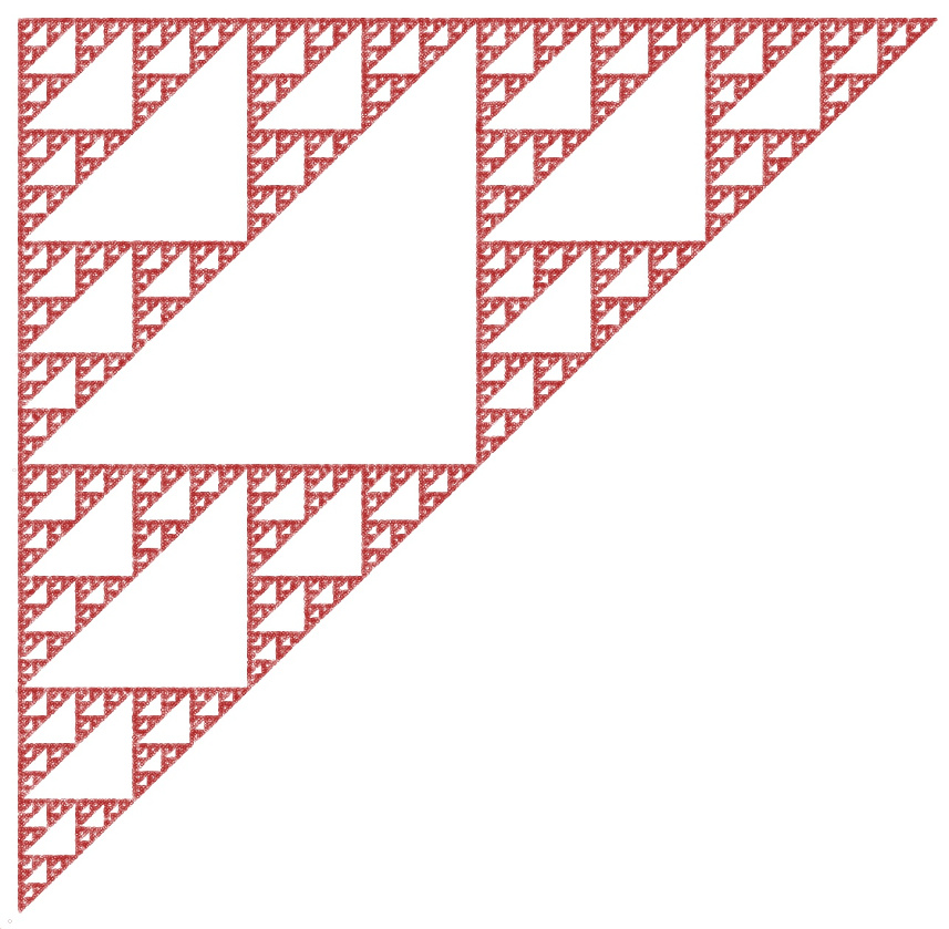
All of these pieces were put together in a Jupyter notebook.  The resulting image is

Note that the Sierpinski Triangle is rotated 45 degrees from the more usual ‘artistic’ expression.  That minor issue is easily rectified using a simple rotation matrix

c45 = 1.0/np.sqrt(2.0)
s45 = 1.0/np.sqrt(2.0)
A   = np.array([[c45,s45],[-s45,c45]])

new_shape = np.array([A.dot(shape[i,:]) for i in range(len(shape))])

where the parameters c45 and s45 are shorthand for $\cos(45 {}^{\circ}) = 1/\sqrt{2}$ and $\sin(45 {}^{\circ}) = 1/\sqrt{2}$, respectively.

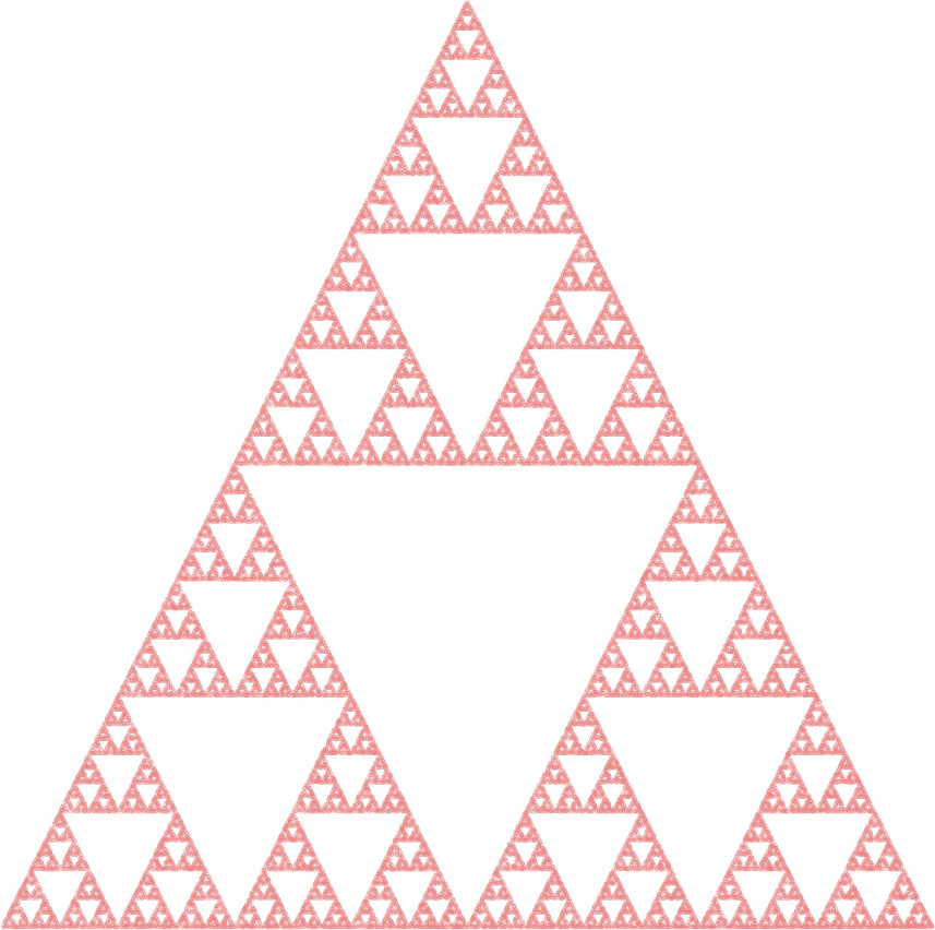
The resulting image is now more aesthetically pleasing.

Making it an equilateral triangle is left as an exercise for the reader.

Note that I’ve played with the color scheme freely and inconsistently from image to image.  Picking and playing with colors is one of the most fun things about exploring the chaos game.

Future columns will look more closely at the chaos game, why it works the way it does and some of the beautiful images that can be produced.

Building on the spirit of whimsy that has been lurking in these columns of late, I thought I would devote one last post to the ambiguities and philosophical twists in natural language.  Not only do these curiosities shed light on the nature of human thought and speech, they also set a standard for any candidate trying to pass the Turing test.  After all, a human response to certain phrases should sometimes be blank confusion or a dumbfounded response like “Sorry, but I don’t have a clue what you mean.”  Other times, subtlety, irony, or humor – all decidedly human expressions – should result when a nuance in language, pointing to an elusive connection, a peculiarity of ideas, or an absurd notion present in a phrase we all take for granted, comes to the front.

The linguistic hedge will be our starting point.  The concept of a linguistic hedge (caution: this Wikipedia link, while containing some useful examples, is full of modern mangling of the language such as using “they” instead of “he” and using passive instead of active voice) is a commonplace and useful component of language that we all use, even if the phrase is unfamiliar.  Suppose you pose the question, “How hungry are you?” to a friend, and his response is, “Very hungry!”; you know that he wants some food fairly badly.  The word “very” is one of the most basic hedges and fuzzy logic often employees it as a mathematical modifier to set membership (maybe more on this in a later post).

People use hedging in a variety of ways, to emphasize degree (as in “very hungry”, or “very, very hungry”), to dodge the truth (as in “to the best of my knowledge”), and to be sarcastic (“she is very good”).  But few uses are as amusing as the use of the word “pretty.”

Ordinarily, English speakers use “pretty” as an adjective, with the typical practice being exemplified by sentences such as “She looks pretty,” or “She looks very pretty.”  However, it is fairly common, in more slang-oriented speech, to say something like “John asked, ‘How big was the rock that you hit with your car?’  Steve answered ‘It was pretty big.’”

Google’s dictionary defines pretty (adverb) as:

Just how does “pretty” turn into a linguistic hedge is a mystery (at least to me) but its use can lead to some very awkward and very funny constructions.  One construction, filled with cleverness and mirth, is the use of pretty to modify words that common speech would normally consider antithetical to the adjectival use of pretty.

For example, there is a comic book published by Image comics called Pretty Deadly.  The book centers on Jenny, the daughter of the embodiment of Death, who is both beautiful and a nearly unstoppable assassin.

An artificial intelligence capable of human-like responses would have to appreciate and, perhaps savor, the double meaning contained in the title, to allow itself to move back and forth between the two separate meanings, to imagine and possibly construct new associations inspired by the juxtaposition of two otherwise dissimilar words.

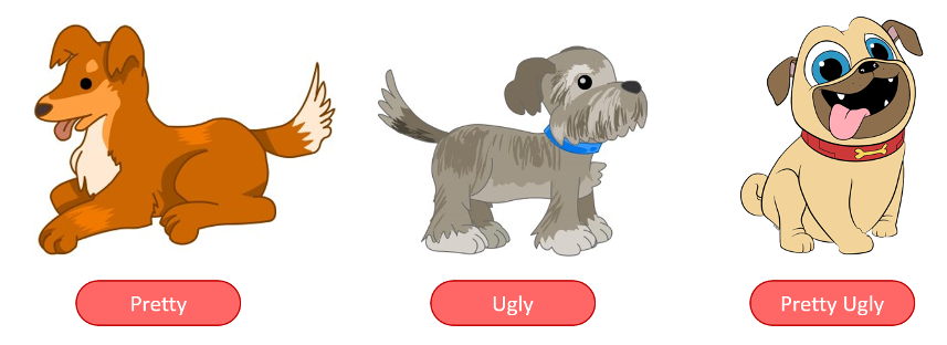
Likewise, to match its biological counterparts, it would have to enjoy the most humorous use of pretty when it modifies adjectives that are exactly opposite to its adjectival form, such as hideous, grotesque, repulsive, and so on.   Consider the following set of man’s best friends

and the fully natural way in which they are labeled.   Imagine an artificial intelligence trying to properly understand why “pretty ugly” or “pretty repulsive” is linguistically intelligible but why “pretty pretty” is just plain wrong.  Of course, one can always program the AI to work around “pretty pretty” as a corner case but take a moment to reflect on who programmed us to recognize just how bad it sounds.  Your answer should have been no one, because we just innately recognize just how stupid that phrase is.

Somehow, a true AI would need to learn and know and imagine how to use linguistic hedges to sound clever or funny or poetic without some vast if-then-else loop or training on large amounts of data that someone else blessed as proper speech.  It should know when to honor the rules and when to break them and when to invent new ones.  But such an AI is nowhere to be seen on the horizon, and that’s pretty sad.

An earlier post (Language and Thought) reflected on the question as if language effects the way we think and if so by how much.  The general conclusion is that the hypothesis that a native speaker can only think thoughts for which his mother tongue possesses a word (the so-called Sapir-Whorf thesis) is unsupported by either common sense or by empirical evidence.  However, there are numerous examples of language shaping the habits and attitudes of its native speakers in interesting and, sometimes, surprising ways.  Attitudes, being what they are, range over the entire gamut of human emotions and the emotional foci for this discussion will be humor and whimsey.

Nothing seems to separate the lower animals from humans as much as the abstract sense of humor.  While mankind shares a sense of pleasure and mirth with more primitive animals no other species exhibits humor in a spoken language littered with abstract concepts, double entendre, and shades of meaning.  A man and a dog may both laugh at someone slipping on a banana peel but only the man will find a ‘man bites dog’ joke funny (although if he does he still qualify as human?).  And if machines will ever get to the point where they can mimic man then they better learn to tell a good joke or, at least, laugh at one.

Topping the list of mirthful, silly constructions, is the buffalo grammar.  For those unfamiliar, a short summary is in order.  The word buffalo can be used as a noun (i.e. the large herd animal also known as a bison), an adjective (as in the city of Buffalo), and as a verb (meaning to fool, puzzle, baffle of mystify).  This flexibility allows English speakers to create all sorts of sentences consisting solely of that one word.

Some examples will help to illustrate.  (Note that a given sentence may have multiple meanings only one of which is used in the illustration.)

1 word:

2 words:

3 words:

4 words:

5 words:

The following youtube video gives more background (although they use another definition for buffalo as a verb – to intimidate or bully).

Far funnier is the video by Cleardino that maps a 8-buffalo-long sentence eventually into Japanese dogs in Tokyo doing unspeakable things to each other.

At the heart of all the mischief caused by all these bison is the concept of lexical ambiguity in which words with multiple senses or meanings can produce sentences and similar structures that are just flat out funny (and confusing).

In 2006, author Lynne Truss provided another wonderfully colorful and beautifully ambiguous string to add to one’s lexicon:  Eats Shoots & Leaves.  The subtitle of the work The Zero Tolerance Approach to Punctuation reveals that her true purpose is to guard society against ‘plummeting punctuation standards’ but for this work we will concentrate on the pandas (giant pandas actually) that gracefully adorn her cover – or at least as gracefully as pandas can do anything.

Depending on the punctuation, specifically the placement of commas, and context different meanings can be wrung from those three innocent words.

For example, suppose the panda in question is currently incarcerated in what animal rights activists may characterize as a gulag-for-lower-life-forms but which you and I may end up calling a zoo.  Faced with the problem of panda nutrition when may be inclined to bring our black-and-white inmates eats, shoots, and leaves meaning food from the local pub (eats), bamboo shoots, and the leaves from a particular nice tree over on the west side of the cage.

Further suppose that an expert on mammalian physiology with a specialty in primates and having world-class expertise in pandas comes by while we are trying to feed one of our bouncing bears potato chips.  He may disgustingly shake his head and yell ‘eats shoots and leaves’ meaning ‘that bear consumes plant shoots and tree leaves’.

Furthermore, suppose that our panda, now aware of our shabby treatment, pulls a loaded revolver (but from where) and ends our miserable existence.  At the inquest, there may be a witness who describes what he saw, in present tense so as to increase the vividness of his description, by saying:

meaning that the panda ate a bite, pulled a gun and shot us, and then skedaddled back to China since there are no extradition agreements that will bring him to justice in the US.

Clearly Truss intends us to take punctuation so seriously that she is willing to use humor to drive her points home.

And lest the reader thinks that this kind of fun is confined only to English consider the following very old and venerated poem in Chinese.

This kind fun (and confusion) makes natural language a real challenge for machine intelligence.  For now, systems are barely able to translate language constructions intended to be clear and communicative.  So it seems a safe bet to say that AI has a long way to go before it is impishly playing with the language.  But when it does, that’s when we should start worrying or maybe laughing, I just don’t know.

It is an often-stated and, I think, well-established idea in the physical sciences that the ‘mathematical words’ used to express an idea are often as important as—or, in certain circumstances, more important than—the ideas being expressed.  ‘Notation matters’ is the catchphrase, and it reflects the belief that better ways of encapsulating an idea lead to better ideas (see e.g. S.S. Chern’s Differential Geometry; Its Past and Its Future).  Basically, the mathematical words used either enable or limit the thoughts that can be conceived or expressed.

The poster child for this belief is the emergence of vector calculus as the language used in field theories.  The physical idea that no magnetic monopoles exist in nature is much harder to see in component form

\[ \frac{\partial B_x}{\partial x} + \frac{\partial B_y}{\partial y} + \frac{\partial B_z}{\partial z} = 0 \]

than in the more compact

\[ \vec \nabla \cdot \vec B = 0 \; .\]

The same argument seems to be widely held in computing.  Certain programming languages (LISP or one of its dialects) are often said to shape how a programmer actually thinks about programming.  Proponents of object-oriented or functional programming maintain that it is easier to express algorithms in these paradigms because they allow the programmer to abstract more complex ideas, thus being able to focus on the logic without being bogged down in the day-to-day syntax.

These ideas have plenty of anecdotes supporting them (and, perhaps, some scientifically gathered and analyzed data) and it is natural to wonder if the same holds true for natural languages; does one’s mother tongue limit the thoughts that one can think?

The simple answer is no.  The mathematical experience teaches us that new ideas can be expressed with the old words, but the result is that we often do so by adding new words to encapsulate these ideas.  In terms of the example above, the compact expression $\vec \nabla \cdot \vec B$ allows one to think more broadly about the magnetic field in the abstract, but the ‘clunky’ coordinate expression is what one uses when one wants to actually compute something.

Nonetheless, philosophers and linguists are not inclined to trust experiences from mathematicians and scientists, and they’ve looked into this point on their own.  After all, the traditional overlap between thought and speech traces its origin back to the ancient philosophers, who regarded the ability to speak as a hallmark indicating that man is a rational animal.  However, the modern renaissance seems to date from 1940 with the work of Benjamin Lee Whorf.

In his article Does Your Language Shape How You Think?, Guy Deutshcer of the New York Times discusses Whorf’s 1940 article entitled Science and Linguistics, which claimed that language imposes a different form of reality on one set of speakers versus another.  As Deutshcer relates, Whorf asserted that, if a language didn’t have a word for a concept, the concept would be unknown to speakers of this language.  It is hard to believe that this assertion was really what Whorf believed or, if so, that it was taken seriously, as there is a reductio ad absurdum argument that would deduce that sentences with multiple words used to express complex ideas would never be needed or used, except to make new words.

Nevertheless, Deutshcer provides some interesting ‘refutations’ of the Sapir-Whorf thesis (Edward Sapir was Whorf’s teacher).  For example, some languages, like Chinese, don’t have a formally delineated future tense whereas English does.  And yet the two sentences “Are you coming tomorrow?” (more Chinese-like) and “Will you come tomorrow?” (less Chinese-like) are equivalent, suggesting that considerations about the future for a native Chinese speaker are not different from those whose native tongue is English, even if they express themselves differently.  Likewise, English didn’t have a single word equivalent for schadenfreude, but English-speakers still indulged in that behavior, and that word has essentially been incorporated into English.

Despite the fact that Whorf’s main conclusions seem to have been wrong, the notion that language shapes thoughts in addition to thoughts shaping language does seem to have some truth.  Deutscher quotes the linguist Roman Jakobson as saying that “languages differ essentially in what they must convey and not in what they may convey”.  To get a sense of what that means, he presents the sentence “I spent yesterday with a neighbor.”, which in English leaves the sex of the neighbor entirely unspecified whereas German, French, or Spanish require the speaker to specify a gender.

Joshua Hartshorne, writing for Scientific American, explores some other aspects in his article Does Language Shape What We Think?  He presents the interesting case of the Pirahã, who have no precise counting words, just general notions.  When asked to exchange, say, seventeen rocks for an equivalent number of sticks, the Pirahã can match the objects one-to-one but they can’t count out seventeen sticks abstractly to prepare the exchange in advance.  Does this behavior suggest that, since they don’t have a word for the abstract idea of seventeen, they don’t know what seventeen is?  Hartshorne doesn’t think so—neither do I.  They just don’t have any abstraction for the counting process.  This is a common problem that English speakers encounter for incredibly large numbers.  I don’t know what a trillion dollars looks like or can buy but I do know how to abstractly denote it in symbols.

In her article Does Language Affect Thought?, Karen Lewis also explores the Sapir-Whorf thesis.  The primary example she discusses centers around mass nouns.  Mass nouns are nouns like mass, water, snow, meat, beer versus count nouns such as chair, pencil, one fish, two fish, red fish, blue fish.  According to Lewis, Whorf maintained that the Hopi had no mass nouns and so they perceived the world differently than we do.  She cites several experiments that suggest that, while the presence or absence of mass nouns in a language influences how the world is linguistically categorized, there is no evidence that the language influences how the speaker conceptualizes the world.

That said, it is clear that language shapes the attitudes, emotions, and preconceptions of its speakers.  In languages with gendered nouns, the adjectives used to describe these nouns depend on the gender of the noun.

What can we conclude from all these examples (and the others found in the articles cited above)?  I think the safest thing to say is that the language we speak doesn’t inhibit us from thinking new thoughts for which we don’t have pre-existing words.  But it can shape how we feel, how quickly we process thoughts, and how we express ourselves.  In a nutshell, underneath we are all the same even if we express ourselves quite differently.

Two earlier posts (An A* Drama and A Cross-Country A*) introduced the A* algorithm, how it manages to find the shortest path (more on this below), and how it can also handle terrain costs.  This post was meant to cover a minor point that was purposely omitted until now.

Unfortunately, this post must also serve as a mea culpa in which I need to apologize for a gross error in my previous two explanations.  The error became apparent as I worked up this column for last month’s installment and the discovery of the error derailed that post in favor of the one on compression and the pigeon hole principle.

In the previous two A* posts, the explanation stated that the scoring of the spots placed on the open list consisted of two parts: 1) the terrain cost (the cost to move onto the spot) and 2) the heuristic cost (an estimate of how far the spot is from the goal).  I forgot to include the total cost from the starting space, which is the sum total of all the movement costs to get to that spot.  Tracking that cost is vital to performing the re-parenting step that takes out any ‘kinks’ in the path that result from random choices the algorithm must make when picking between two spots of equal cost.

Despite this omission, the algorithm actually performed quite well in the two cases examined and it found the shortest pay in the wayfarer example (A Cross-Country A*) where the terrain costs were the primary driver and no obstacles were present.  It fared slightly worse in the original example with the angry snake and the man who poked him (An A* Drama), finding almost the shortest path, being only one step too long.  Sadly, that error escaped my notice for some time.

Fortunately, the error came and presented itself quite clearly when I returned to the snake v. man drama to explain re-parenting.   To see what re-parenting involves consider this step in the snake’s pursuit of his vengeance.

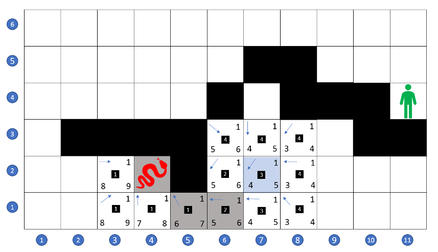
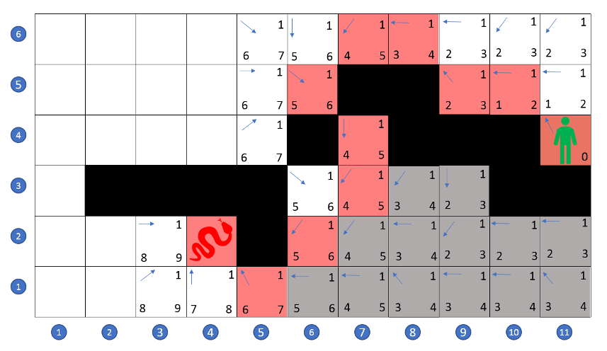
Faced with two spaces, (7,1) and (7,2), with the same total cost of 8 – 1 for terrain (upper right) and 4 for the heuristic (lower left), for a movement cost of 5 (lower right), and a cost of 3 steps from the starting space (black square in the center) – the snake randomly chooses to explore gird space (7,2).  Doing so opens up (i.e. places on the open list) spots (7,1), (8,1), (6,2), (8,2), (6,3), (7,3), and (8,3), parents them all to (7,2), and scores them all as having a total cost from the starting space of 4, since any path to these spaces must first go through (7,2), which is 3 steps away from the starting space.

The key point to note, is that the shortest path from the starting space to spaces (6,3) and (7,3) (for a total cost from start of 3) passes through spot (6,2), which is not explored first because of its greater cost.  As a result, the current path to either (6,3) or (7,3) first goes past them to the right while it approaches from below before going back to the left as it arrives; the last three spots in the path are connected as (6,1) -> (7,2) -> (6,3).  Because of its shape, I call such a sub-optimal path a kink.

Now that we recognized the kink, what are we to do with it?  Well, for the time being we just let it alone.  When the algorithm finally explores one of these points, we simply look to see if shifting its parent from (7,2) to some other nearby space will lower the total cost from the starting spot.  If so, then the parent is changed and the algorithm continues essentially unchanged.

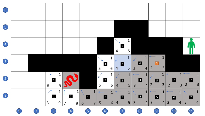
To be concrete, consider the situation a bit further in the snake’s search for a path to his foe.  After meandering in the lower right for a while, the snake’s exploration has carried him to space (7,3), which, as a reminder, has received a total cost from the start space of 4 and which is parented to (7,2).

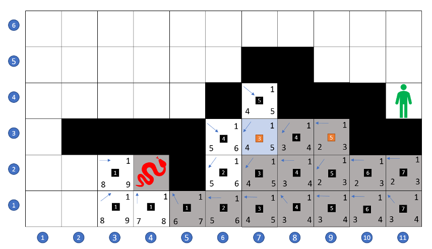
As the snake explores space (7,3), he looks around to see if re-parenting the space to any of the neighboring spaces will lower the total cost from the starting space.  He notes that re-parenting (7,3) to (6,2) will lower that total cost from the starting space by 1 and he does so.  The box containing the new cost has been colored orange to reflect this change.

Because (7,4) had been opened and scored when (8,3) was explored, it also will be re-parented when the snake recognizes the strategic importance of slithering through (7,4).

The final path requires the snake to make 10 steps to reach his victim.

It is a matter of a few minutes of playing with other paths to convince oneself that this is the smallest cost to wreak his revenge.  Of course, the path passing through (6,3) -> (7,4) is equally short but won’t be found by the A* since the heuristic scoring tends to pull the paths to the right even though the ‘escape route’ requires moving to the left.  Also note, that without re-parenting, the kink would have cost an extra step, driving the total cost to 11.

So, there you have it.  A corrected and complete presentation of the A* algorithm.  Sorry for the confusion, but, at least, the error helped to frame the importance of re-parenting in finding the shortest path.

This month’s column was meant to be an additional exploration of the A* algorithm but, as the old saying goes, the best laid plans of mice and men… and so on.   So that exploration is going to have to wait until a later column. But deadlines being deadlines, and commitments being commitments, I thought I would offer a tongue-in-cheek discussion about two serious subjects.

The first subject is the logically based, mathematically provable theorem called the pigeonhole principle.  On its surface, the pigeonhole principle says an entirely obvious fact that if one has $$n$$ objects into $$m$$ holes, where $$n>m$$, then you must, necessarily, have at least one hole with more than one object in it.

When first encountering this statement, everyone’s initial reaction is “Of course! That’s obvious!” but the full extent of all the implications of this statement often takes some time to get used to and some people never grasp the scope.

One of the more interesting blind-spots concerns file compression.  An amazingly large number of people, spread across the entire societal cross-section, believe that any file can be losslessly compressed.  They may not assert that categorically but they are often surprised when they find out that a lossless compression algorithm can actually make the ‘compressed’ size bigger (for example consider this post).

By definition, lossless compression is a process that replaces the bit pattern in a file with another bit pattern such in such a way that the original can be recovered from the new pattern by inverting the process.  When a losslessly compressed file is smaller than the original, it means that blocks of the information in the file are redundant.  In simplistic terms, there are patterns of bits that are sufficiently large that they can be replaced with a smaller pattern of bits.

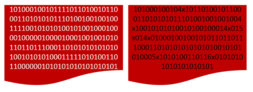
Ignoring for the moment the restriction that a file must be represented by bits (equivalently, ignoring exactly how to implement the following) a lossless compression could take the bit field ‘100000010111111’ and replace it with ‘16x0106x1’, where the string ‘6×0’ means ‘000000’.  This is an example of tokenizing the data and ‘6×0’ is a token – a string that stands in for another.  This process is completely invertible and, for a field of even modest size, can make the resulting file smaller.

Unfortunately, the pigeonhole principle guarantees that the process can’t be repeated indefinitely.  If the bit pattern is sufficiently random, the tokenization process can actually result in a bit pattern larger than the original file.  This is typically encountered when trying to compress an already compressed file.

The mathematical proof of this is not something worth presenting.  Rather, there is a slick reductio ad absurdum argument that is easier to understand, a lot more satisfying, and leaves a punch line in its wake.

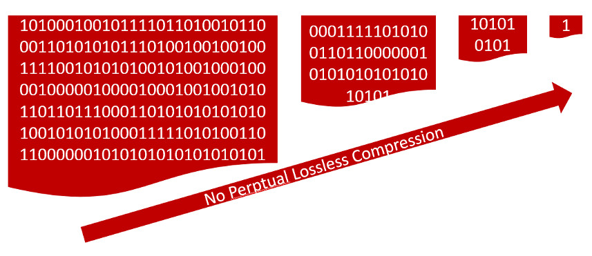
Imagine the same file as before and further imagine that lossless compression results in a file smaller by some factor (for convenience a factor of 4 was used in the following figure) after each application.  The first compressed file then becomes the source for the second, the second for the third, and so on.  Eventually, the original file should be able to be characterized by a single very interesting bit.  Since we reject that idea, we must conclude that at some stage the compression fails to compress.

So, it is clear that lossless compression can’t make every file smaller.  Now call that file where the lossless compression fails to compress the base file (or the devil’s file, if you like to be dramatic).  Since that bit pattern clearly contains all the information we want (either it is the original or it is one the files that results by applying the lossless compression) in a pattern that can’t be made smaller, then the only file that can be as small as it is one with the exact same bit pattern; any other file must be bigger.  Since the lossless compression produces a new bit pattern, it must necessarily be bigger.

Now onto the next principle.  There is no official name for it nor is it a principle on par with the pigeonhole principle.  It is not based on logic or mathematics or computer science but on common sense and experience with human nature.  For the sake of argument in this blog, it will be called the no-bug principle.

Quite simply stated, the no-bug principle asserts that no piece of code of sufficient size/complexity is truly free of bugs no matter how many people or how much money and time a group spends on eliminating them.

Like its more rigorously proven cousin, the no-bug principle strikes disbelief into the hearts of people from all walks of life.  The usual manifestation of this disbelief is the eye-rolling and snark-filled rants that come from otherwise rational people when a glitch is encountered in a favorite app or program.  The duration of the rant and its intensity are inversely proportional to the amount of coding experience the ranter has.  Typical utterances include things like “I can’t believe they didn’t test this before they shipped” or “I could do better than this $%@^$” and similar statements vomited out under duress.

Ironically, these ranters are also typically the people who sue for pardon in their own work and defend themselves with statements like “well, if I had more time” or “nobody’s perfect”.

Interestingly, the two principles can be combined in comic fashion if we reject the first and accept the second.  Recognizing that any executable is simply a pattern of bits, we can then comfort ourselves in believing that every executable can be reduced to a single very interesting bit that is filled to the brim with bugs.

Last month’s column introduced and explored the basic A* algorithm within the cheeky context of a snake, a man, and a path to revenge.  In this month’s post, the algorithm is extended to include terrain costs that take into account that different types of spots may be more expensive to traverse based on their nature (e.g., mountain, river, forest, desert, etc.).  As in the simpler case already studied, the A* seeks to find the shortest path between a starting point and the goal when the latter is known but the best way to travel is not.

It is important to remember that at the core of the A* algorithm is the idea of an open spot.  An open spot is a location adjacent to the current spot that the algorithm is visiting.  From the vantage of the current spot, the neighboring spots can be examined and scored based on two criteria:  the cost to move into that spot and a heuristic guess as to how far the spot is from the goal.  These actions open the spot, which is placed on a list for future exploration.  Once the A* has finished examining the neighborhood of the current spot, it closes that spot and selects the next spot to visit from among the lowest scoring spots on the list of open spots.  By keeping pointers from open spots to the parent spots that opened them, the A* is able to back-track from the goal (once it has found it) to the beginning spot, thus determining the shortest path.  The reader is encouraged to read the earlier post (An A* Drama) for more details.

As in the previous post, the material here is strongly influenced by Chapter 7 of AI for Game Developers, by David M. Bourg and Glenn Seemann.

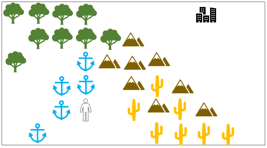
This month’s story begins with a wayfarer, who is journeying in the wilderness, looking for the shortest path home to his city.

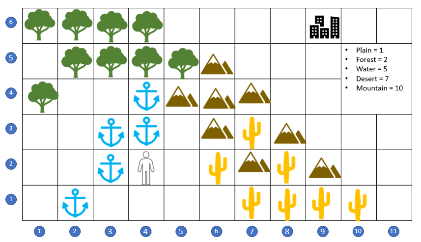
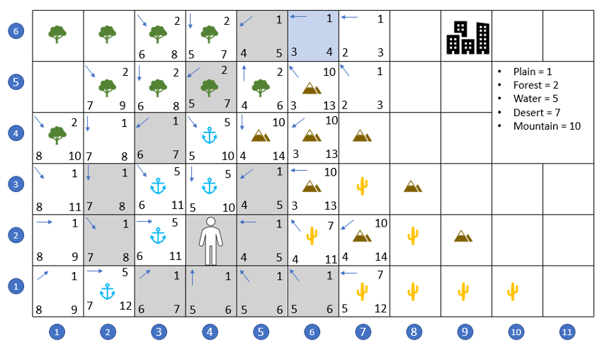
He weighs his options for path based not just on distance but on how well he can travel across each type of terrain.   Normalizing his speed to the plain (blank of unfilled space), the wayfarer estimates that he can move 2 faster across the plain than through the forest, 5 times faster than crossing the water, 7 time faster than moving across the desert, and 10 times faster than climbing over the mountains.  To evaluate his options he records his travel-time estimates and then lays a grid over his map to assist with his planning.

The mountain range to his north-east lies in a direct, as-the-crow-flies path from his current location at grid point (4,2) to the city at (9,6), but taking this route may not be the most time-optimal approach.  He starts looking for ways to go around rather than over the mountain range.

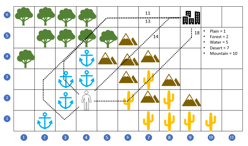
By going through the desert to the east and south-east, he can head in roughly the ‘right’ direction and skirt the mountains completely, but the desert is not much cheaper than the mountains.  He also considers going due north along the river course and then turning east in the forest, but a river trip is 5 times slower than in the plain.  Finally he considers the possibility of going in the completely ‘wrong’ direction by heading to the south-west, where a ford allows him to cross the river on foot.  Once on the other side, he can follow the flow upstream (to the north-east) until he enters the forest and can approach the city from the east.  He scores these different possibilities and find that the last route is the cheapest.

Given the same information, will the A* also find this over-the-river-and-through-the-woods path?

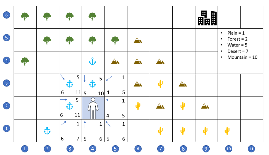
The first step to answering this question is to add the terrain cost to the A* algorithm.  This is done by simply using the time-scaling the wayfarer had already noted to the local score when a spot is opened.    For example, when the search begins, the A* starts at (4,2) and opens the 8 locations surrounding that spot.  Grid locations (4,3), (3,3), and (3,2) are assigned a local cost of 5 since they are river spots.  The remaining five spots ((3,1), (4,1), (5,1), (5,2), and (5,3)) are assigned a local cost of 1 since they are plain spots.

The heuristic scoring for the remaining cost is calculated as it was in the previous case as simply the as-the-crow-flies distance; that is to say that no regard is paid to terrain cost or even if the spot is available for traversal.  It turns out that as long as all spots are scored on even footing with a common heuristic, the details of the scoring don’t matter.

Initially, the A* flirts with moving to the north-east since the local costs are low (being plains) and the total cost is low since the path is moving in the correct direction.  But quickly, the A* loses interest in these paths since their score, once opened, places them near the bottom of the open list.

After some exploration, the A* settles in on the path across the river, up along the western shore, through the forest to the north, and straight on to the east, thus bypassing the mountains and desert completely.

At this point, the A*, can pick either (7,5) or (7,6) as the next spot with no penalty, since both take the same amount of time in this geometry.  The selection for equally-scored spots is random so A* can meander a bit picking between any of the following paths:

• (6,6) -> (7,6) -> (8,6) -> goal (9,6)
• (6,6) -> (7,6) -> (8,5) -> goal (9,6)
• (6,6) -> (7,5) -> (8,5) -> goal (9,6)
• (6,6) -> (7,5) -> (8,6) -> goal (9,6),

since they are all equivalent.  For simplicity, I’ve coaxed the A* into the first of the list paths in the movie below but as far as our wayfarer is concerned, he gets home as safely by relying on A* as he does by his own skills as a world-weary traveler.

I suppose this blog post started first with some analysis I had decided to do on the A* algorithm and then it just grew from there.  I had employed the A* algorithm on a scheduling problem some years back.  This application was advocated by one of the developers on my team but I didn’t have the time to properly learn it during development and deployment.  I ended up using it as a black box with a silent vow to get around to learning it one of these days.

Years passed, and my son was learning it as part of a course he was taking and I thought now was the time.  So, I purchased AI for Game Developers, by David M. Bourg and Glenn Seemann and dug into Chapter 7 entitled A* Pathfinding.  If you happen to read their book, you’ll find that the approach is highly influenced by and patterned after their material.  To my credit, I slogged through a complete example and then animated in a nice little video.  If you are interested in that, it can be found at the bottom of this post.

The premise of the A* algorithm is that the starting point and ending point for some sort of journey are known but that the specific path from A-to-B, as it were, is not.  The personal picture I like to entertain is embarking on a car trip from New York to Los Angeles.  I know where I am starting and I know where I am to finish, but should I drive through Pennsylvania or Maryland or further south?  Does Kentucky figure into my route?  What about Idaho?  And so on.  The hope is to find the shortest path that connects the start with the end with only a general notion of how far apart the two are.

For simplicity, let’s consider a much simpler problem of a snake trying to find the man who poked him while he dozed on a warm rock in the summer sun.

Our slithering protagonist abstracts the terrain and lays down a grid, with himself starting at the grid point (4,2).  He sees that the man is at the grid point (11,4) so he begins to formulate his revenge.  However, being impatient to return to his sun-bathed nap our hero wants to dispatch the man as soon as possible.  He needs the shortest path.  Being mathematically minded and knowledgeable about algorithms, he decides on using the A* algorithm.

The A* algorithm consists of the following steps:

1. Assume that the starting spot is open
2. Take a look around at the nearest neighbor spots
3. If they can be occupied, open them by
   1. Putting them on the open list for subsequent visit
   2. Score them with a perceived cost to move onto them
   3. Score them with an estimated cost representing how far they are from the destination square
   4. Total the two scores to give a total cost for the spot
   5. Assign a pointer from the open spot to the parent spot
4. If they can’t be occupied (e.g. the are boundaries or forbidden) ignore them
5. Close the starting spot
6. Pick the lowest cost open spot on the list (picking arbitrarily if there are ties)
7. Open and score any unopened spot
8. Close the spot and repeat

If one of the open spots is the destination spot, don’t bother scoring it (i.e. give it a score of 0) and back-track from it to the start, following all the pointers.  The resulting path can then be traversed in the forward fashion.

For the simple example examined here, the perceived cost will be taken to be 1 for all possible spots, meaning the speed with which any spot can be crossed is the same.  In general, spots own a terrain cost that may make it more or less expensive than neighboring spots (the difference between a highway and a surface street each with dramatically different speed limits).

The estimated cost is evaluated using a heuristic that counts the spots between the open spot and the final spot with no regard to barriers or terrain.

Returning to our intrepid reptile, his spot at (4,2) is now shaded blue, meaning it is in the process of being closed.  He scores the spots at (3,2), (3,1), (4,1) and (5,1) and finds that the total costs are 9, 9, 8, and 7 respectively (the heuristic cost for (4,1) is 8 because it takes eight moves, horizontally, vertically, or diagonally to get to (11,4)).

Of the four spaces he has now opened, he selects (5,1) to next consider as its cost of 7 is the lowest of the bunch.   Spot (4,2) is now closed (shaded gray) and examining spot (5,1) then opens spots at (6,1) and (6,2).

Each of these has a score of 6 so he arbitrarily picks (6,1) to examine, opening the additional spots at (7,1) and (7,2).  Again, he picks arbitrarily between these two spots, since both own a score of 5 and are the cheapest members of the open list.

His full adventure can be found in the video below, including a frame-by-frame look at just how he tries to put his revenge in motion.  Spoiler:  the man gets what’s coming to him in the end.