In the last post, we examined the Holt-Winter scheme for tracking the level, trend, and seasonal variations in a time series in a sequential fashion with some synthetic data designed to illustrate the algorithm in as clean a way as possible. In this post, we’ll try the Holt-Winter method against real world data for US housing sales and will set some of the context for why the method works by comparing it to a related technique called the moving average.
The data analyzed here were obtained from RedFin (https://www.redfin.com/news/data-center/) but it isn’t clear for how long RedFin will continue to make these data public as they list the data as being ‘temporarily released’. As a result, I’ve linked the data file I’ve used here.
We’re going to approach these data in two ways. The first is by taking a historical look at the patterns in the data from the vantage point of hindsight on the entire span of home sales having been collected. In the second approach, we imagine what an agent working in the past thinks as the data come in one record at a time.
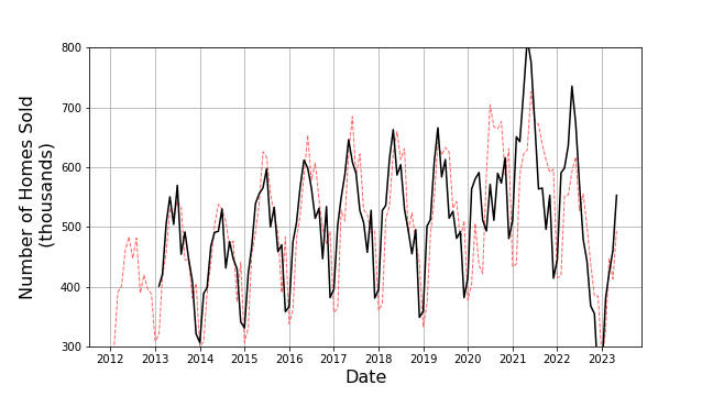
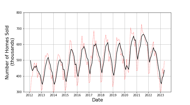
The historical look starts with an overview of the number of homes sold in the time period starting in Feb 2012 and ending at May 2023.

These data show both seasonal and overall trend variations and so our expectation might be that Holt-Winter would do a good job but note two things: First, with the exception of the first pandemic year of 2020, each of the years shows the same pattern: sales are low in the winter months and strong in the summer ones. Second the trend (most easily seen by focusing on the summer peak) shows four distinct regions: a) from 2012-2017 there is an overall upward trend, b) from 2017-2020 the trend in now downward with a much shallower slope, c) the start of the pandemic lockdowns in 2020 breaks the smoothness of the trend and then the trend again has a positive slope over 2020-2021, and d) the trend is strongly downward afterwards. These data exhibit a real-world richness that the contrived data used in the last post did not and they should prove a solid test for a time series analysis agent/algorithm.
Depending on how ‘intelligent’ we want our analysis agent to be we could look at a variety of other factors to explain or inform these features. For our purposes, we’ll content ourselves with looking at one other parameter, the median home sales price, mostly to satisfy our human curiosity.
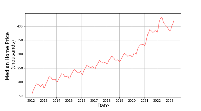
These data look much more orderly in their trend and seasonal variation over the time span from 2012-2020. Afterwards, there isn’t a clear pattern in terms of trend and season.
Our final historical analysis will be to try to understand the overall pattern of the data using a moving average defined as:
\[ {\bar x}_{k,n} = \frac{1}{n} \sum_{i =k-n/2}^{k+n/2} x_i \; . \]
The index $k$ specifies to which point of the underlying and $n$ the number of points to be used in the moving average. Despite the notation, $n$ is best when odd so that there are as many points before the $k$th one as there are after as this prevents the moving average from introducing a bias which shifts a peak in the average off of the place in the data where it occurs. In addition, there is an art in the selection of the value of $n$ between it being too small, thereby failing to smooth out unwanted fluctuations, and being too large which smears out the desired patterns. For these data, $n = 5$. The resulting moving average (in solid black overlaying the original data in the red dashed line) is:
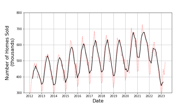
Any agent using this technique would clearly be able to describe the data as having a period of one year with a peak in the middle and perhaps an overall upward trend from 2012 to 2022 but then a sharp decline afterwards. But two caveats are in order. First and the most important one, the agent employing this technique to estimate a smoothed value on the $k$th time step must wait until at least $n/2$ additional future points have come in. This requirement usually precludes being able to perform predictions in real time. The second is that the moving average is computationally burdensome when $n$ is large.
By contrast, the Holt-Winter method can be used by an agent needing to analyze in real time and it is computationally clean. At the heart of the Holt-Winter algorithm is the notion of exponential smoothing where the smoothed value at the $k$th step, $s_k$, is determined by the previous smoothed value $s_{k-1}$ and the current raw value $x_k$ according to
\[ s_k = \alpha x_k + (1-\alpha) s_{k-1} \; . \]
Since $s_{k-1}$ was determined from a similar expression at the time point $k-1$, one can back substitute to eliminate all the smoothed values $s$ on the right-hand side in favor of the raw ones $x$ to get
\[ s_k = \alpha x_k + (1-\alpha)x_{k-1} + (1-\alpha)^2 x_{k-2} + \cdots + (1-\alpha)^k x_0 \; . \]
This expression shows that the smoothed value $s_k$ is a weighted average of all the previous points making it analogous to the sequential averaging discussed in a previous post but the exponential weighting by $(1-\alpha)^n$ makes the resulting sequence $s_k$ look more like the moving average. In some sense, the exponential smoothing straddles the sequential and moving averages giving the computational convenience of the former while providing the latter’s ability to follow variations and trends.
How closely the exponentially smoothed sequence matches a given $n$-point moving average depends on the selection of the value of $\alpha$. For example, with $\alpha = 0.2$ the exponentially smoothed curve gives
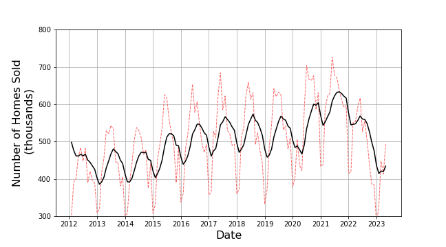
whereas $\alpha = 0.4$ gives
Of the two of these, the one with $\alpha=0.4$ much more closely matches the 5-point moving average used above.
The Holt-Winter approach using three separate applications of exponential smoothing, hence the need for the three specified parameters $\alpha$, $\beta$, and $\gamma$. Leslie Major presents an method for optimizing the selection of these three parameters in her video How to Holts Winters Method in Excel & optimize Alpha, Beta & Gamma.
We’ll skip this step and simply use some values informed by the best practices that Major (and other YouTubers) note.
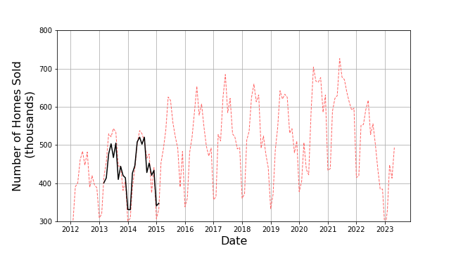
The long-term predictions given by our real time agent are pretty good in the time span 2013-2018. For example, a 24-month prediction made in February 2013 looks like
Likewise, a 24-month prediction in June 2017 looks like
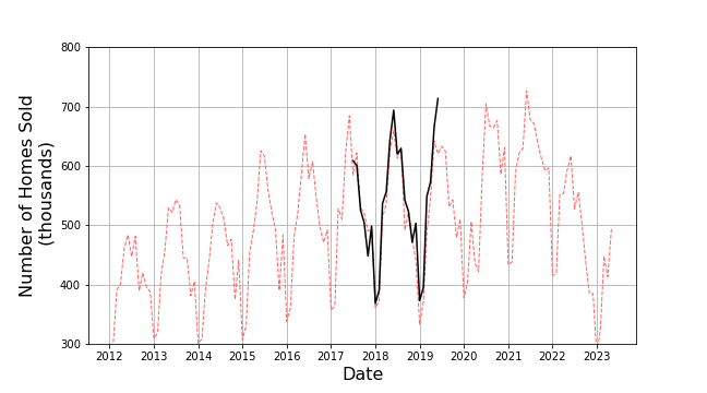
Both have good agreement with a few areas of over or under-estimation. The most egregious error is the significant overshoot in 2019 which is absent in the 12-month prediction made a year later.
All told, the real time agent does an excellent job of predicting in the moment but it isn’t perfect as is seen by how the one-month predictions falter when the pandemic hit.