
A hallmark of intelligence is the ability to anticipate and plan as events occur as time elapses. Evaluating and judging each event sequentially is how each of us lives but, perhaps ironically, this is not how most of us are trained to evaluate a time series of data. Typically, we collect quantitative and/or qualitative data for some time span, time tagging the value of each event, and then we analyze the entire data set in as one large batch. This technique works well for careful, albeit leisurely, exploration of the world around us.
Having an intelligent agent (organic or artificial) working in the world at large necessitates using both techniques – real time evaluation in some circumstances and batch evaluation in others – along with the ability to distinguish when to use one versus the other.
Given the ubiquity of time series in our day-to-day interactions with the world (seasonal temperatures, stock market motion, radio and TV signals) it seems worthwhile to spend some space investigating a variety of techniques for analyzing these data.
As a warmup exercise that demonstrates the differences between real time and batch nuances involved, consider random numbers pulled from a normal distribution with a mean ($\mu = 11$) and standard deviation ($\sigma = 1.5$).
Suppose that we pull $N=1000$ samples from this distribution. We would expect that the sample mean, ${\bar x}$, and sample deviation $S_x$ to be equal to the population mean and standard deviation to within 3% (given that $1/\sqrt(1000) \approx 0.03$). Using numpy, we can put that expectation to the test, finding that for one particular set of realizations that the batch estimation over the entire 1000-sample set is ${\bar x} = 11.08$ and $S_x = 1.505$.
But how would we estimate the sample mean and standard deviation as points come in? With the first point, we would be forced to conclude that ${\bar x} = x_0$ and $S_x = 0$. For subsequent points, we don’t need to hold onto the values of the individual measurements (unless we want to). We can develop an iterative computation starting with the definition of an average
\[ {\bar x} = \frac{1}{N} \sum_{i=1}^N x_i \; .\]
Separating out the most recent point $x_N$ and multiplying the sum over the first $N-1$ points by the $1 = (N-1)/(N-1)$ gives
\[ {\bar x} = \frac{N-1}{N-1} \frac{1}{N} \left( \sum_{i=1}^{N-1} x_i \right) + \frac{1}{N} x_N \; .\]
Recognizing that the first term contains the average ${\bar x}^{(-)}$ over the first $N-1$ points, this expression can be rewritten as
\[ {\bar x} = \frac{N-1}{N} {\bar x}^{(-)} + \frac{1}{N} x_N \; .\]
Some authors then expand the first term and collect factors proportional to $1/N$ to get
\[ {\bar x} = {\bar x}^{(-)} + \frac{1}{N} \left( x_N – {\bar x}^{(-)} \right) \; .\]
Either of these iterative forms can be used to keep a running tally of the mean. But since the number of points in the estimation successively increases as a function of time, we should expect that difference between the running average and the final batch estimation to also be a function of time.
While there is definitive theory that tells us the difference between the running tally and the population mean there isn’t any theory that characterizes how it should rank relative to the batch estimation other than the generic expectation that as the number of points used in the running tally approaches the number in the batch estimation that the two should converge. Of course, the final value must exactly agree as there were no approximations made in the algebraic manipulations above.
To characterize the performance of the running tally, we look at a variety of experiments.
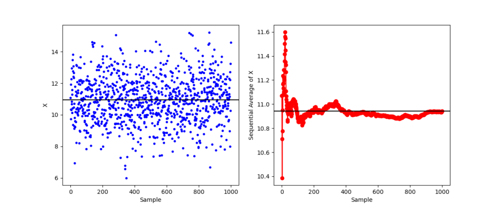
In the first experiment, the running tally fluctuates about the batch mean before settling in and falling effectively on top.
But in the second experiment, the running tally starts far from the batch mean and (with only the exception of the first point) stays above the until quite late in the evolution.
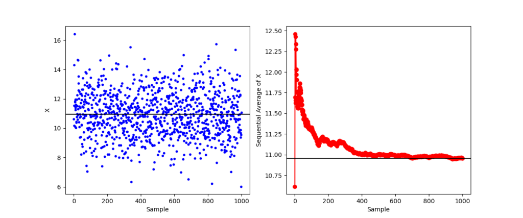
Looking at the distribution of the samples on the left-hand plot shows that there was an overall bias relative to the batch mean with a downward trend, illustrating how tricky real data can be.
One additional note, the same scheme can be used to keep a running tally on the average of $x^2$ allowing for a real time update of the standard deviation from the relation $\sigma^2 = {\bar {x^2}} – {\bar x}^2$.
As the second case demonstrates, our real time agent may have a significantly different understanding of the statistics than the agent who can wait and reflect over a whole run of samples (although there is a philosophical point as to what ‘whole run’ means). In the months to come we’ll explore some of the techniques in both batch and sequential processing.