Latest Posts

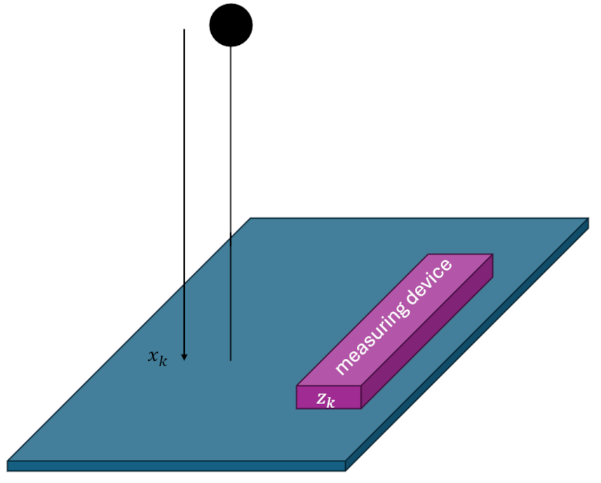
A Symbolic Experiment – Part 1:  First Expression

One of the most active areas of artificial intelligence in the earlier days (say from 1960s through the 1990s) was the development of symbolic AI to handle mathematical manipulations.  In his book, Paradigms of Artificial Intelligence Programming: Case Studies in Common Lisp, Peter Norvig covers numerous applications that were solved as the ‘hot’ topics of the day; a time before the before the advent of deep learning came along and convinced most people that LLM’s and agentic systems would solve all the world’s problems.  However, these former hot topics are still relevant today and I thought that it might be interesting to explore a bit to see what can be done with ‘old fashioned’ symbolic manipulation.

There are three reasons for embarking on this exploration. 

First, understanding the nuts and bolts of symbolic manipulation makes one a better user of the ‘professional’ computer algebra systems (CASs) on the market today, such as wxMaxima, Maple, Mathematica, and SymPy.  Each of these is polished and abstracted (to varying degrees) and seeks to help the user, typically a mathematician, scientist, or engineer, in making a model and subsequently applying it to some specific problem.  However, each of these systems (especially the for-profit ones), want the user to be able to solve problems immediately without, necessarily, knowing how the CAS works behind the scenes.  While these systems are quite powerful (again to lesser or greater degrees), experience has shown that most users don’t/can’t take full advantage of the system unless they can program in it.  And to program in it requires a firm understanding of at least the rudiments of what is happening under the hood.  This is a sentiment Norvig emphases repeatedly in his book, most notably by providing the following quote:

You think you know when you learn, are more sure when you can write, even more when you can teach, but certain when you can program.

Alan Perlis, Yale University computer scientist

Second, there are always new mathematics being invented with brand new rules.  Being able to manipulate/simplify and then mine an expression for meaning transcends blindly applying a built-in trig rule like $\cos^2 + \sin^2 = 1$, a generic ‘simplify’ method, or some such thing.  It often requires understanding how an expression is formed and what techniques can be used to take an expression apart and reassemble as something more useful.

Third, and finally, it’s fun – plain and simple – and most likely will be a gateway activity for even more fun to come.

Not that we’ve resolved to explore, the next choice is which part of terra incognita.  The undiscovered country that I’ve chosen is the implementation of a simple set of symbolic rules, via pattern matching, that implement some of the basic properties of the Fourier Transform.

For this first experiment, I chose Sympy as the tool of choice as it seemed a natural one since it provides the basic machinery of symbolic manipulation for free in Python but it doesn’t have a particularly sophisticated set of rules associated with the Fourier Transform.  For example, SymPy version 1.14 knows that the transform is linear but it doesn’t know how to simplify the Fourier Transform based on the well-known rule:

\[ {\mathcal F}\left[ \frac{\partial f(t)}{\partial t} \right] = i \omega {\mathcal F}\left[ f(t) \right] \; , \]

which is one of the most important relationships for the Fourier Transform as it allows us to convert differential equations into algebraic ones, which is one of the primary motivations for employing it (or any other integral transform for that matter).

Before beginning, let’s set some notation.  Functions in the time domain will be denoted by lower case Latin letters (e.g., $f$, $g$, etc.) and will depend on the variable $t$.  The corresponding Fourier Transform will be denoted by upper case Latin letters (e.g., $F$, $G$, etc.) and will depend on the variable $\omega$.  Arbitrary constants will also be denoted by lower case Latin letters but usually from the beginning of the alphabet (e.g., $a$, $b$, etc.). The pairing between the two will be symbolically written as:

\[ F(\omega) = {\mathcal F}(f(t)) \; ,\]

with an analogous expression for the inverse.  The sign convention will be chosen so that the relationship for the transform of the derivative is as given above.

For the first experiment, I chose the following four rules/properties of the Fourier Transform:

  1. Linearity:  ${\mathcal F}(a \cdot f(t) + b \cdot g(t) ) = a F(\omega) + b G(\omega)$
  2. Differentiation: $\mathcal{F}\left[\frac{d^n f(t)}{dt^n}\right] = (i \omega)^n F(\omega)$
  3. Time Shifting:  $\mathcal{F}{f(t – t_0)} = e^{-i \omega t_0} F(\omega)$
  4. Frequency Shifting: $\mathcal{F}{e^{i \omega_0 t} f(t)} = F(\omega – \omega_0)$

We expect freshman or, at worst, sophomores in college to absorb and apply the rules above and, so, we may be inclined to think that they are ‘straightforward’ or ‘boring’ or ‘dull’.  But, finding a way to make a computer do algorithmically what we expect teenagers to pick up from a brief lecture and context is surprisingly involved. 

Our hypothetical college student’s capacity to learn, even when not explicitly taught is an amazing and often overlooked miracle of the human animal.  Unfortunately, teaching any computer to parse ‘glyphs on a page’ in a way that mimics what a person does requires a lot of introspection into just how the symbols are being interpreted.  Mathematical expressions are slightly easier as they tend to have less ‘analogical elasticity’; that is to say, that by their very nature, mathematical terms and symbols tend to be more rigid that everyday speech.  More rigid doesn’t mean completely free of ambiguities as the reader may reflect on when thinking about what the derivatives in the Euler-Lagrange equations actually mean:

\[ \frac{d}{dt} \left( \frac{\partial L}{\partial {\dot q}} \right) – \frac{\partial L}{\partial q} = 0 \; . \]

Let’s start with a simple mathematical expression that is needed for the Linearity property

\[ a \cdot f(t) +  b \cdot g(t) \; . \]

When composing this expression, a person dips into the standard glyphs of the English alphabet (10 of them to be precise) and simply writes them down.  If pressed, the person may go onto say “where $a$ and $b$ are constants and $f$ and $g$ are, as yet undefined functions of the time variable $t$”.  But the glyphs on the page remain all the same.  For a computer, are the glyphs ‘a’ and ‘b’ of the same type as the glyphs ‘f’ and ‘g’?  And where does ‘(t)’ figure in? 

SymPy’s answer to this (which matches most of the other CASs) is that ‘a’, ‘b’, and ‘t’ are Symbols and ‘f’ and ‘g’ are undefined Functions.  The bold-face terms are syntactically how SymPy creates these symbolic objects. These objects can be used as ordinary Python objects with all the normal Python syntax (e.g., print(), len(), type(), etc.) coming along because SymPy tries to strictly adhere to the Python data model.  As a result, we can form new expressions by using ‘+’ and ‘*’ without worrying about how SymPy chooses to add and multiply it various objects together.

The following figure shows the output of a Jupyter notebook that implements these simple steps.

As expected, querying type(a) gives back sympy.core.symbol.Symbol and type(f) returns sympy.core.function.UndefinedFunction.  And, as expected, we can form our first expression

my_expr = a*f(t) + b*g(t)

from using ‘+’ and ‘*’ as effortlessly as we wrote the analogous expression above out of basic glyphs, without having to worry about details.  But what to make of type(my_expr) returning sympy.core.add.Add?

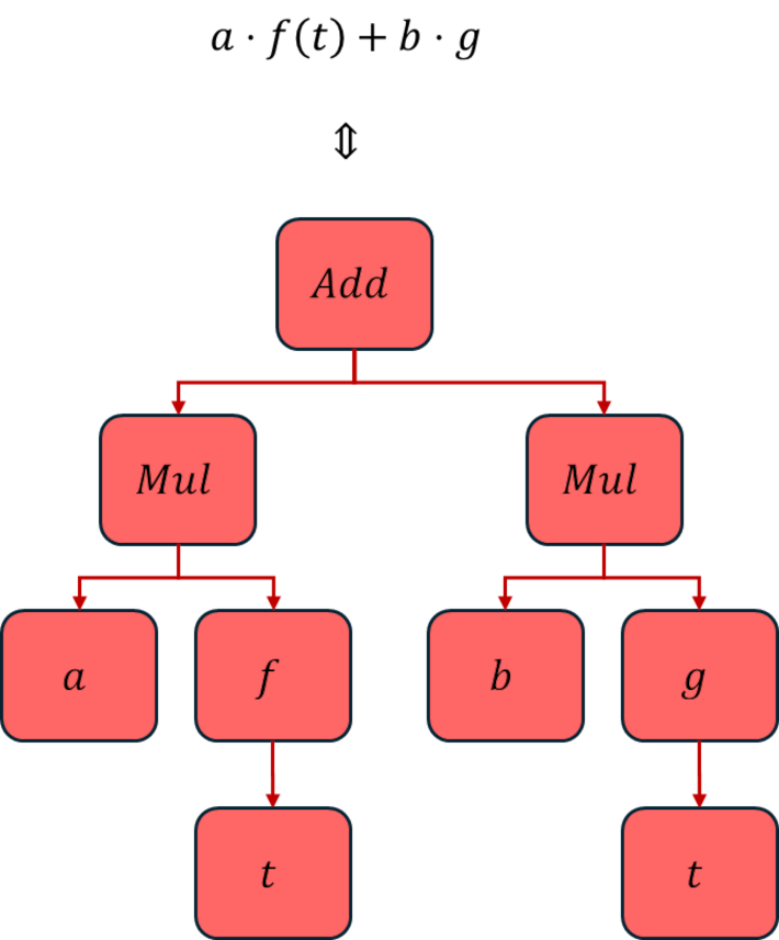
The answer to this question gets at the heart of how most (if not all) CASs work.  What we humans take for granted as a simple expression $a \cdot f(t) + b \cdot g(t)$ is, for SymPy (and all the other CASs that I’ve seen), a tree.  The top node is this case is Add meaning that ‘+’ is the root and each of the two subexpressions ($a \cdot f(t)$ and $b \cdot g(t)$) are child nodes, each of type sympy.core.mul.Mul.  SymPy symbols are atomic nodes that can only be root nodes or child nodes but can never serve as parent nodes.  And the distinction between the Symbol and Function objects are now much clearer: giving a glyph the designation as a Function means it can serve as a parent node, even if all of its behavior is, as yet, undefined.

The innocent-looking expression from above has the tree-form

Next month, we’ll continue on to show how to examine, traverse, and modify this tree structure so that we can mimic how a human ‘plays with’ and ‘mine meaning from’ an expression.

Time Series 6 – Recursive Least Squares

The last post introduced the notion of the recursive least squares estimation approach as a natural precursor to the Kalman filter and derived the Kalman-like gain that governed the state estimation update equation.  Before moving on to a simple example of the Kalman filter, it seemed prudent to show the recursive least squares filter in action with a numerical example.

The example involves a mass falling in an unknown uniform gravitational field with unknown initial conditions.  At regular time intervals, a measurement device measures the height of the mass above the ground but only to within certain precision due to inherent noise in it measuring processes.  The challenge is then to deliver the best estimate of the unknowns (initial height, initial speed, and the uniform gravitational acceleration).   We will assume that, beyond a measurement of the initial height, the other initial conditions are inaccessible to the measurement device since it only measures range.  This example is adapted from the excellent article Introduction to Kalman Filter: Derivation of the Recursive Least Squares Method by Aleksander Haber.

To prove that the recursive least squares method does generate a real least squares estimation, let’s first look at how a batch least squares approach to this problem would be performed.

The dynamics of the falling mass are given by

\[ d(t) = d_0 + v_0 t + \frac{1}{2} a t^2 \; , \]

where $d(t)$ is the height above the ground at a given instant.

We assume that the above equation is exact; in other words, there are no unknown forces in the problem.  In the language of Kalman-filtering and related optimal estimation, there is said to be no process noise, with it understood that the word ‘process’ is a genetic umbrella meaning the dynamics by which the state evolves in time, for which Newton’s laws are an important subset.

By design, measurements come in every $\Delta t$ seconds and so the time evolution of the fall of the mass is sampled at times $t_k = k \Delta t$.  At measurement time $t_k$ the amount the mass has dropped is

\[ x_k = x_0 + v_0 k \Delta t + \frac{1}{2} k^2 \Delta t^2  a \; \]

and the corresponding measurement is

\[ z_k = x_k + \eta_k \; , \]

where $\eta_k$ is the noise the measuring device introduces in performing its job.

The batch least squares estimation begins by writing the evolution equation in a matrix form

\[ z_k = \left[ \begin{array}{ccc} 1 & k \Delta t & \frac{1}{2} k^2 \Delta t^2 \end{array} \right] \left[ \begin{array}{c} x_0 \\ v_0 \\ a \end{array} \right]  + \eta_k \equiv H_{k,p} x_p + \eta_k \; .  \]

The array $x_p$ contains the constant initial conditions and unknown acceleration that is being estimated.

For this numerical experiment, $x_0 = -4m$, $v_0 = 2 m/s$ (positive being downward), and $a = 9.8 m/s^2$ the usual value for surface of the Earth (give or take regional variations).  Measurements are taken every $\Delta t = 1/150 s$ over a time span of 14.2 seconds.  To illustrate the meaning of $H_{k,p}$, the value of the matrix at $k=0$ is

\[ H_{k=0,p} = \left[ \begin{array}{ccc} 1 & 0 & 0 \end{array} \right] \; \]

corresponding to an elapsed time of $t_k = 0$ and at $k = 75$

\[ H_{k=0,p} = \left[ \begin{array}{ccc} 1 & 0.5 & 0.125 \end{array} \right] \; \]

corresponding to an elapsed time of $t_k = 0.5$. 

The merit of this matrix approach is that by putting every measurement into a batch we can write the entire measured dynamics in a single equation as:

\[ z = H x + \eta \; . \]

The array $z$ has $M$ elements (for the number of measurement), where $M$ is the maximum value of the time index $k$ (for this specific example $M$ = 2131).  The matrix $H$ is a $M \times n$ where $n$ is the number of estimate parameters ($n$ = 3, in this case) and $x$ is the array of parameters to be estimated).  The array $\eta$ represents the $M$ values of random noise (assumed to be stationary) that were present in the measurements.  The values of $\eta$ used in this numerical example were drawn from a normal distribution with a zero mean and a standard deviation of 1; the latter value determines the value of $R_k = 1$.

Since, in the matrix equation above, the matrix $H$ isn’t square, it may not be obvious how to solve for $x$.  However, there is a well-known technique using what is known as the Moore-Penrose pseudoinverse

In short, to solve for $x$ in a least squares sense, we set $\eta$ to zero (i.e., we ignore the noise assuming the classical argument that with enough measurements the influence of the noise will average to zero).  We then left-multiply by the transpose of $H$ to get

\[ H^T z = (H^T H) x \; .\]

The quantity $H^T H$ is a $(n \times K) \cdot (K \times n) = n \times n $ matrix (in this case $3\times 3$, which is invertible.  We then arrive at the compact form of the estimate for $x$ as

\[ x_{est} = (H^T H)^{-1} H^T z \; .\]

For this numerical experiment, the resulting estimate is

\[ x_{est} = \left[ \begin{array}{c} -3.95187658 \\ 1.99300377 \\ 9.80040125  \end{array}    \right] \; .\]

This is the same value one gets by using a package like numpy’s linalg.lstsq.

In the recursive method, all of the data are not stored and handled at once but rather each point is taken and processed as it comes in. 

The algorithm developed in the last post is summarized as:

  • Start each step with the current time $t_k$, measurement $z_k$, and the previous estimates of the state $x_{k-1}$ and the covariance $P_{k-1}$
  • Perform the $k$-th calculation of the gain: $K_k = P_{k-1} \cdot H_k^T \cdot S_k^{-1}$, where $S_k = H_k \cdot P_{k-1} \cdot H_k^T + R_k$
  • Make the $k$-th estimate of the unknowns: ${\hat x}_k = {\hat x}_{k-1} + K_k \left( z_k – H_k {\hat x}_{k-1} \right)$
  • Make the $k$-th update of the covariance matrix: $P_k = \left(I – K_k H_k \right)P_{k-1} $

Using this algorithm, the time evolution of the estimated initial position is

with a final value of -3.95170034.

Likewise, the time evolution of the estimated initial speed is

with a final value of 1.99295453.

And, finally, the time evolution of the estimated acceleration is

with a final value of 9.80040698.

These estimated values, up to the numerical noise introduced by a different set of floating point operations, are identical with the batch least squares numbers.

Time Series 5 – Deriving a Kalman-like Gain

Last month’s blog presented one of the most common approaches to handling time series data in real time known as the Kalman gain.  As noted, the form of the state update equations is formally

\[ x_{new} = x_{old} + K ( obs_{new} – obs_{pred} ) \; , \]

where $x$ is the state being estimated and $obs$ is some observation made of the state.  The subscripts on the observation terms are ‘new’ for the latest actual observation (made by some instrument) and ‘pred’ for what the expected predicted observation would be before we made it. 

For the sequential or running average discussed in the first of these series of posts, this general form specifies as

\[ {\bar x} = {\bar x}^{-} + \frac{1}{N} \left( x_N – {\bar x}^{-} \right) \; , \]

where ${\bar x}$ is the estimated average.  For exponential smoothing (and, by extension Holt-Winter), discussed in the third of these series of posts, the general form becomes

\[ s_k = s_{k-1} + \alpha \left( x_k – s_{k-1} \right) \; , \]

where $s_k$ is the smoothed form of some time-varying quantity $x_k$.  For Kalman filtering, discussed in the fourth of these series of posts, the general form takes on the appearance of

\[ {\hat x}_k = {\hat x}_k^{-} + K_k \left( z_k – H {\hat x}_k^{-} \right) \; , \]

where ${\hat x}_k$ is the revised estimated state at time $t_k$ based on the difference between the current measurement $z_k$ and the a priori estimated state ${\hat x}_k^{-}$ at the same time. 

The ‘magic’ in all these cases lies firmly in determining the ‘gain’ that sits outside the difference between the new observation datum and the expected value of the same based on the previous estimate. 

In running average and Holt-Winter cases, it is fairly easy to deduce the form of the gain without any formal mathematical manipulations.  A few rearrangements and some intuition serve.  In the case of the Kalman filter a lot more effort is involved.

As a stepping-stone exercise which has almost all of the ingredients found in the Kalman filter but is both easier to understand and slightly easier to manipulate is the recursive least squares estimator.  The presentation below is strongly influenced by the excellent article Introduction to Kalman Filter: Derivation of the Recursive Least Squares Method by Aleksander Haber with mathematical simplifications gleaned from the Wikipedia entry on the Kalman Filter

Haber’s system of equations models a process in which a constant set of parameters are unknown but can be estimated from a time series of measurements of a time-varying state whose evolution is solely determined by the set of parameters.  The measurement equation is given by

\[ z_k = H_k x + v_k \; . \]

The time varying matrix $H_k$ serves to map the constant but unknown state $x$ forward in time.  The term $v_k$ represents the measurement noise, which is assumed to be zero-mean Gaussian distributed with a covariance given by

\[ E[v_k v_k^T ] = R \; .\]

The concrete example that Haber provides is an object being subjected to constant acceleration starting from an unknown initial position and speed.  The object’s motion obeys

\[ x(t) = x_0 + v_0 t + \frac{1}{2} a t^2 =  \left[ \begin{array}{ccc} 1 & t & \frac{1}{2} t^2 \end{array} \right] \left[ \begin{array}{c} x_0 \\ v_0 \\ a \end{array} \right]  \equiv H(t) x \; .\]

The conversion from the continuous process matrix $H(t)$ to the discrete time-sampled $H_k$ is trivially done by noting that the time $t_k = k \Delta t$. 

Haber claims that a least squares estimation of $x$ can be determined recursively by the process

\[ x_k = x_{k-1} + K_k ( z_k – H_k x_{k-1} ) \; , \]

where $x_k$ is the current estimate of $x$, $z_k$ is the current measurement, and in which the gain $K_k$ will be given by the optimality condition that we want to minimize the error.

To find the explicit form of the gain, we first define the error in state estimation as

\[ \epsilon_k = x – {\hat x}_k \; . \]

Since the parameter set is generically multi-dimensional we will want to minimize the total error

\[ W = E[(\epsilon_k)_1^2] + E[(\epsilon_k)_2^2]+ \ldots + E[(\epsilon_k)_i^2] \; , \]

where the expectation is over all possible realizations of the random error in the measurement.  If we form the covariance matrix of the error

\[ P_k = E[ \epsilon_k \epsilon_k^T] \; \]

then the total error is trace of the covariance matrix: $W = Tr(P)$.  Taking the derivative of this trace and setting it equal to zero provides the explicit form for the gain as follows.

First, re-express the current estimation error in terms of the previous time estimation and via the update equation

\[ \epsilon_k = x – x_{k-1} – K_k(z_k – H_k x_{k-1}) \;  .\]

Using the measurement equation, current estimation error becomes

\[ \epsilon_k = x – x_{k-1} – K_k( H_k x + v_k – H_k x_{k-1} ) \; .\]

This last form re-emphasizes that, in the absence of the measurement noise $v_k$, the determination of the unknown parameter set $x$ would be exact since all the quantity in the parentheses would be identically zero.

Regrouping the terms so that the state variables are gathered separately from the noise yields

\[ \epsilon_k = (1 – K_k H_k) (x – x_{k-1}) – K_k v_k \equiv T_k (x – x_{k-1}) – K_k v_k \; . \]

Now it relatively easy to right multiply the above expression by its transpose

\[ \epsilon_k \epsilon_k^T = T_k (x – x_{k-1} ) (x – x_{k-1} )^T T_k^T + K_k v_k v_k^T K_k^T \\ – K_k v_K (x – x_{k-1} )^T T_k^T – T_k (x – x_{k-1} ) v_k^T K_k^T \; \]

and take an expectation of it to arrive at the covariance matrix

\[P_k = E[ (T_k (x – x_{k-1}) (x – x_{k-1})^T T_k^T]  – E[K_k v_k v_k ^T K_k^T] \; . \]

The cross-terms between the state and the measurement noise vanish under the assumption that the noise is zero-mean distributed (i.e., unbiased). 

Since $K_k$ and $H_k$ only depend on the time-independent value of the noise covariance $R$, they can be factored out of the expectation and we arrive at

\[ P_k = (1 – K_k H_k) P_{k-1} (1 – K_k H_k)^T + K_k R K_k^T \; , \]

which is the Joseph form of covariance propagation relating the covariance matrix at time $t_k$ to one at an earlier time $t_{k-1}$.

The last step is to take the trace and minimize it.  While there are a number of formulae for doing this step that engineers and mathematicians favor, it is easier to use index notation since it frees one from the bother of finding the correct formula and then applying it.

To proceed, expand the Joseph form term-by-term and define $S_k = H_k P_{k-1} H_k^T + R$, to get

\[ P_k = P_{k-1} – K_k H_k P_{k-1} – P_{k-1} H_k^T K_k^T + K_k S_k K_k^T \; . \]

Now, we can suppress the indices on the right since we know that every matrix bears a $k$ subscript except any covariance matrix, which must have a $k-1$ subscript.

The trace is then given by

\[ Tr(P_k) = P_{ii} – K_{ij} H_{j\ell} P_{\ell i} – P_{ij} C_{j\ell}^T K_{\ell i}^T + K_{ij} S_{j \ell} K_{\ell i} \; .\]

The least squares minimization is expressed as

\[ \frac{\partial Tr(P_k)}{\partial K_{st}} = 0 \; . \]

The derivative on the left can be expressed as

\[ \frac{\partial Tr(P_k)}{\partial K_{st}} = – H_{t \ell} P_{\ell s} – P_{sj}H_{jt}^T + S_{t \ell} K_{\ell s}^T + K_{sj} S_{jt} \; .\]

Re-arranging the terms and indices (subject to the transposes) to return to a matrix-multiplication form, yields

\[ \frac{\partial Tr(P_k)}{\partial K} = – 2 P_{k-1} H_k^T + K_k (S_k + S_k^T) \; , \]

where the $k$ index has been restored once the matrix indices have been suppressed.

The last step is to recognize that

\[ S^T = (H P H + R)^T = (H^T)^T P^T H^T + R^T = H P H^T + R \; \]

since both the state and noise covariance matrices are symmetric.

The final step is to set all of that equal to zero and solve to $K_k$.  Doing so gives

\[ K_k S_k = P_{k-1} H_k^T \; , \]

which immediately solves to

\[ K_k = P_{k-1} H_k^T S_k^{-1} = P_{k-1} H_k^T \left[ H_k P_{k-1} H_k^T + R \right]^{-1} \; .\]

Next blog, we’ll explore a numerical example of this method and establish that it does deliver the least squares estimation of the parameter set $x$.

Time Series 4 – Introduction to Kalman Filtering

This month we turn from the exponential smoothing and moving average techniques for analyzing time series and start a sustained look at the Kalman filter.  The Kalman filter has been hailed as one of the most significant mathematical algorithms of the 20th century.  The primary reason for this praise is that the Kalman filtering enables a real time agent to make mathematically precise and supported estimates of some quantity as each data point comes in rather than having to wait until all the data have been collected.  This enabling behavior garners Kalman filtering a lot of attention and Russell and Norvig devote part of their chapter on probabilistic reasoning in their textbook Artificial Intelligence: A Modern Approach to it.

Before diving into the mathematical details, it is worth noting that the thing that sets the Kalman filter apart from the Holt-Winters algorithm is that in the latter, we needed to recognize and characterize a reoccurring pattern in our data.  For example, in the Red Fin housing sales, the data are conveniently regularly spaced in monthly intervals and seasonal patterns are readily apparent if not always predictable.  The Kalman filter imposes no such requirements, hence its usefulness.  It is often used in navigation activities within the aerospace field where it is applied to powered flight of a missile as readily as to a low-Earth orbiting spacecraft like Starlink to a libration orbiting spacecraft like JWST.

There are an enormous number of introductions to the Kalman filter each of them with their own specific strengths and weakness.  I tend to draw on two works: An Introduction to the Kalman Filter by Greg Welch and Gary Bishop and Poor Man’s Explanation of Kalman Filtering or How I stopped Worrying and Learned to Love Matrix Inversion by Roger M. du Plessis.  The latter work is particularly difficult to come by, but I’ve had it around for decades.  That said, I also draw on a variety of other references which will be noted when used.

I suppose there are four core mathematical concepts in the Kalman filter:  1) the state of the system can be represented by a list of physically meaningful quantities, 2) these quantities vary or evolve in time in some mathematically describable way, 3) some combination (often nonlinear) of the state variables may be measured, 4) the state variables and the measurements of them are ‘noisy’.

Welch and Bishop describe these four mathematical concepts as follows.  The state, which is described by a $n$-dimensional, real array of variables

\[ x \in \mathbb{R}^n \; \]

evolves according to the linear stochastic differential equation

\[ x_k = A x_{k-1} + B u_{k-1} + w_{k-1} \; , \]

where $A$, which is known as the $n \times n$ real-valued process matrix, provides the natural time evolution of the state at earlier time $t = k-1$ to the state at time $t = k$.  The quantity $u \in \mathbb{R}^{\ell} $ is a control or forcing term that is absent in the natural dynamics but can be impose externally on the system.  The $n \times \ell$, real-valued matrix $B$ maps the controls into the state evolution.  The term $w \in \mathbb{R}^n$ is the noise in the dynamics; it typically represents those parts of the natural evolution or of the control that are either not easily modeled or are unknown.

Measurement of the state is represented an $m$-dimensional, real-valued vector $z \in \mathbb{R}^m$ and is related to the state by the equation

\[ z_k = H x_k + v_k \; , \]

where $H$ is a $m \times n$ real-valued matrix and $v \in \mathbb{R}^m$ is the noise in the measurement.

In addition, both noise terms are assumed to be normally distributed with their probabilities described by

\[ p(w_k)  = N(0,Q_k) \; \]

and

\[ p(v_k) = N(0,R_k) \; , \]

where $Q_k \in \mathbb{R}^{n \times n}$ is the process noise covariance matrix and $R_k \in \mathbb{R}^{m \times m}$ is the measurement noise covariance matrix.  We further assume that they are uncorrelated with each other.  Generally, these noise covariances are time-varying since their values typically depend on the state.

Note that both the state and measurement equations are linear.  More often than not, Kalman filtering is applied to nonlinear systems but in those cases, the estimation process is linearized and the above equations are used.  Whether that is a good idea or not is a discussion for another day. 

The role of the Kalman filter is to produce the best estimate of the state at a given time given the above equations.  To do so, the filter algorithm draws heavily on concepts from Bayesian statistics to produce a maximum likelihood estimate. 

In terms of Bayesian statistics, the algorithm assumes both an a priori state estimate ${\hat x}^{-}_{k}$ and an a posteriori one ${\hat x}_{k}$.  The transition from the a priori to the a posteriori is made with

\[ {\hat x}_k = {\hat x}^{-}_{k} + K_k (z_k – H {\hat x}^{-}_k ) \; , \]

where the ‘magic’ all happens due to the Kalman gain $K_k$ defined as

\[ K_k = P^{-}_k H^T \left( H P^{-}_k H^T + R \right) ^{-1} \; , \]

where ‘$T$’ indicates a matrix transpose.

Note that this equation is functionally similar to the running average form calculated as

\[ {\bar x} = {\bar x}^{-} + \frac{1}{N} \left( x_N – {\bar x}^{-} \right) \; . \]

We’ll return to that similarity in a future post. 

For now, we will round out the menagerie of mathematical beasts by noting that $P_k$ is the state covariance, a $n \times n$, real-valued matrix, that summarizes the current statistical uncertainty in the state estimation.  Formally, it is defined as

\[ P_k = E \left[ (x_k – {\hat x}_k ) (x_k – {\hat x}_k )^T \right] \; , \]

where the ‘$E$’ stands for expectation over the state distribution. 

The state covariance can be associated with the a priori estimate, where it is denoted as $P^{-}_k$ or with the a posteriori estimate, where it is denoted by $P_k$.  The two are related to each other by

\[ P_k = A P^{-}_k A^T + Q \; . \]

The Kalman algorithm is best summarized using the following flow diagram adapted from the one in Introduction to Random Signals and Applies Kalman Filtering 4th Edition by Brown and Hwang.

In future blogs, we’ll explore how to derive the magical Kalman gain, some applications of it to agent-based time series estimation, and a variety of related topics.  It is worth noting that the notation is fluid, differing from author to author and application to application.

Time Series 3 – Exponential Smoothing and Holt-Winter

In the last post, we examined the Holt-Winter scheme for tracking the level, trend, and seasonal variations in a time series in a sequential fashion with some synthetic data designed to illustrate the algorithm in as clean a way as possible.  In this post, we’ll try the Holt-Winter method against real world data for US housing sales and will set some of the context for why the method works by comparing it to a related technique called the moving average.

The data analyzed here were obtained from RedFin (https://www.redfin.com/news/data-center/) but it isn’t clear for how long RedFin will continue to make these data public as they list the data as being ‘temporarily released’.  As a result, I’ve linked the data file I’ve used here.

We’re going to approach these data in two ways.  The first is by taking a historical look at the patterns in the data from the vantage point of hindsight on the entire span of home sales having been collected.  In the second approach, we imagine what an agent working in the past thinks as the data come in one record at a time. 

The historical look starts with an overview of the number of homes sold in the time period starting in Feb 2012 and ending at May 2023.

These data show both seasonal and overall trend variations and so our expectation might be that Holt-Winter would do a good job but note two things: First, with the exception of the first pandemic year of 2020, each of the years shows the same pattern: sales are low in the winter months and strong in the summer ones. Second the trend (most easily seen by focusing on the summer peak) shows four distinct regions: a) from 2012-2017 there is an overall upward trend, b) from 2017-2020 the trend in now downward with a much shallower slope, c) the start of the pandemic lockdowns in 2020 breaks the smoothness of the trend and then the trend again has a positive slope over 2020-2021, and d) the trend is strongly downward afterwards.  These data exhibit a real-world richness that the contrived data used in the last post did not and they should prove a solid test for a time series analysis agent/algorithm.

Depending on how ‘intelligent’ we want our analysis agent to be we could look at a variety of other factors to explain or inform these features.  For our purposes, we’ll content ourselves with looking at one other parameter, the median home sales price, mostly to satisfy our human curiosity.

These data look much more orderly in their trend and seasonal variation over the time span from 2012-2020.  Afterwards, there isn’t a clear pattern in terms of trend and season. 

Our final historical analysis will be to try to understand the overall pattern of the data using a moving average defined as:

\[ {\bar x}_{k,n} = \frac{1}{n} \sum_{i =k-n/2}^{k+n/2} x_i \; . \]

The index $k$ specifies to which point of the underlying and $n$ the number of points to be used in the moving average.  Despite the notation, $n$ is best when odd so that there are as many points before the $k$th one as there are after as this prevents the moving average from introducing a bias which shifts a peak in the average off of the place in the data where it occurs.  In addition, there is an art in the selection of the value of $n$ between it being too small, thereby failing to smooth out unwanted fluctuations, and being too large which smears out the desired patterns.  For these data, $n = 5$.  The resulting moving average (in solid black overlaying the original data in the red dashed line) is:

Any agent using this technique would clearly be able to describe the data as having a period of one year with a peak in the middle and perhaps an overall upward trend from 2012 to 2022 but then a sharp decline afterwards.  But two caveats are in order.  First and the most important one, the agent employing this technique to estimate a smoothed value on the $k$th time step must wait until at least $n/2$ additional future points have come in.  This requirement usually precludes being able to perform predictions in real time.  The second is that the moving average is computationally burdensome when $n$ is large.

By contrast, the Holt-Winter method can be used by an agent needing to analyze in real time and it is computationally clean.  At the heart of the Holt-Winter algorithm is the notion of exponential smoothing where the smoothed value at the $k$th step, $s_k$, is determined by the previous smoothed value $s_{k-1}$ and the current raw value $x_k$ according to

\[ s_k = \alpha x_k + (1-\alpha) s_{k-1} \; . \]

Since $s_{k-1}$ was determined from a similar expression at the time point $k-1$, one can back substitute to eliminate all the smoothed values $s$ on the right-hand side in favor of the raw ones $x$ to get

\[ s_k  = \alpha x_k + (1-\alpha)x_{k-1} + (1-\alpha)^2 x_{k-2} + \cdots + (1-\alpha)^k x_0 \; . \]

This expression shows that the smoothed value $s_k$ is a weighted average of all the previous points making it analogous to the sequential averaging discussed in a previous post but the exponential weighting by $(1-\alpha)^n$ makes the resulting sequence $s_k$ look more like the moving average.  In some sense, the exponential smoothing straddles the sequential and moving averages giving the computational convenience of the former while providing the latter’s ability to follow variations and trends.

How closely the exponentially smoothed sequence matches a given $n$-point moving average depends on the selection of the value of $\alpha$.  For example, with $\alpha = 0.2$ the exponentially smoothed curve gives

whereas $\alpha = 0.4$ gives

Of the two of these, the one with $\alpha=0.4$ much more closely matches the 5-point moving average used above. 

The Holt-Winter approach using three separate applications of exponential smoothing, hence the need for the three specified parameters $\alpha$, $\beta$, and $\gamma$.  Leslie Major presents an method for optimizing the selection of these three parameters in her video How to Holts Winters Method in Excel & optimize Alpha, Beta & Gamma

We’ll skip this step and simply use some values informed by the best practices that Major (and other YouTubers) note.

The long-term predictions given by our real time agent are pretty good in the time span 2013-2018.  For example, a 24-month prediction made in February 2013 looks like

Likewise, a 24-month prediction in June 2017 looks like

Both have good agreement with a few areas of over or under-estimation.  The most egregious error is the significant overshoot in 2019 which is absent in the 12-month prediction made a year later. 

All told, the real time agent does an excellent job of predicting in the moment but it isn’t perfect as is seen by how the one-month predictions falter when the pandemic hit.

Time Series 2 – Introduction to Holt-Winter

In the last blog, I presented a simple sequential way of analyzing a time series as data are obtained.  In that post, the average of any moment $x^n$ was obtained in real-time by simply tracking the appropriate sums and number of points seen.  Of course, in a real world application, there would have to be a bit more intelligence built into the algorithm to allow an agent employing it to recognize when a datum is corrupted or bad or missing (all real world problems) and to exclude these point both from the running sums and from the number of points processed. 

This month, we look at a more sophisticated algorithm for analyzing trends and patterns in a time series and for projecting that analysis into the future sequential using these patterns.  The algorithm is a favorite in the business community because, once an initial ‘training’ set has been digested, the agent can update trends and patterns with each new datum and then forecast into the future.  The algorithm is called the Holt-Winter triple exponential smoothing and it has been used in the realm of business analytics for forecasting the number of home purchases, the revenue from soft drink sales, ridership on Amtrak, and so on, based on a historical time series of data.

Being totally unfamiliar with this algorithm until recently, I decided to follow and expand upon the fine video by Leslie Major entitled How to Holts Winters Method in Excel & optimize Alpha, Beta & Gamma.  In hindsight, this was a very wise thing to do because there are quite a few subtle choices for initializing the sequential process and the business community focuses predominantly on using the algorithm and not explaining rationale for the choices being followed.

For this first foray, I am using the ‘toy’ data set that Majors constructs for this tutorial.  The data set is clean and well-behaved but, unfortunately, is not available from any link discernable associated with the video but I have reconstructed it (with a lot a pauses) and make it available here

The data are sales $W$ of an imaginary item, which, in deference to decades of tradition, I call a widget.  The time period is quarterly and a plot of the definitive sales $W$ from the first quarter of 2003 (January 1, 2003) through the fourth quarter of 2018 (October 1, 2018) shows both seasonal variations (with a monotonic ordering from the first quarter as the lowest to the fourth quarter as the highest)

as well as a definite upward trend for each quarter.

The Holt-Winter algorithm starts by assuming that the first year of data are initially available and that a first guess for a set of three parameters $\alpha$, $\beta$, and $\gamma$ (associated with the level $L$, the trend $T$, and the seasonal $S$ values for the number of widget sales, respectively) are known.  We’ll talk about how to revise these assumptions after the fundamentals of the method are presented.

The algorithm consists of 7 steps.  The prescribed way to initialize the data structures tracking the level, trend, and seasonal values is found in steps 1-4, step 5 is a boot-strap step initialization needed to start the sequential algorithm proper once the first new datum is obtained and steps 6-7 comprise the iterated loop step used for all subsequent data, wherein an update to the current interval is made (step 6) and then a forecast into the future is made (step 7).

In detail these steps require an agent to:

  1. Determine the number $P$ of intervals in the period; in this case $P = 4$ since the data are collected quarterly. 
  2. Gather the first period of data (here a year) from which the algorithm can ‘learn’ how to statistically characterize it.
  3. Calculate the average $A$ of the data in the first period.
  4. Calculate the ratio of each interval $i$ in the first period to the average to get the seasonal scalings $S_i = \frac{V_i}{A}$.
  5. Once the first new datum $V_i$ ($i=5$) (for the first interval in the second period) comes in, the agent then bootstraps by estimating:
    1. the level in the first interval by making a seasonal adjustment.  Since the seasonal level is not yet known, the agent uses the seasonal value in the previous period in the first interval using $L_i = \frac{V_i}{S_{i-P}}$;
    1. the trend of the first interval in the second period using $T_{i} = \frac{V_i}{S_{i-P}} – \frac{V_{i-1}}{S_{i-1}}$.  This odd looking formula is basically the finite difference between the first interval of the second period and the last interval of the first period, each seasonally adjusted.  Again, since the seasonal level is not yet know, the agent uses the seasonal value from the corresponding earlier interval for the first interval of the second period;
    1. the seasonal ratio of the first interval in the second period using $S_i = \gamma \frac{V_i}{L_i} + (1-\gamma) S_{i-P}$.
  6. Now, the agent can begin sequential updating in earnest by using all of the weighted or blended averages of the data in current and past intervals to update:
    1. the level using $L_i = \alpha \frac{V_i}{S_{i-P}} + (1-\alpha)(L_{t-1} + T_{t-1})$
    1. the trend using $T_i = \beta ( L_i – L_{i-1} ) + (1-\beta) T_{t-1}$
    1. the seasonal ratio (again) using $S_i = \gamma \frac{V_i}{L_i} + (1-\gamma) S_{i-P}$
  7. Finally, the agent can forecast as far forward as desired (using $F_{i+k} = (L_i + k \cdot T_i) S_{i – P + k}$. where $k$ is an integer representing the number of ‘intervals’ ahead to be forecasted.  There are some subtleties associated with what the agent can do with a finite number of historical levels of the seasonal ratios, so, depending on application, specific approximations for $S_{i – P + k}$ must be made.

Using the widget sales data, the first 4-quarter forecast compares favorable to the actuals as seen in the following plot.

When forecasting only a quarter ahead, as Major herself does, the results are also qualitatively quite good.

Finally, a note about selecting the values of $\alpha$, $\beta$, and $\gamma$.  There is a general rule of thumb for initial guesses but that the way to nail down the best values is to use an optimizer to minimize the RMS error between a forecast and the actuals.  Majors discusses all of these points and shows how Excel can be used in her video to get even better agreement.

For next month, we’ll talk about the roots of the Holt-Winter algorithm in the exponential smoother (since it is applied to three parameters – level, trend, and seasonal ratio – that is why the algorithm is often called triple exponential smoothing).

Time Series 1 – Sequential Averaging

A hallmark of intelligence is the ability to anticipate and plan as events occur as time elapses.  Evaluating and judging each event sequentially is how each of us lives but, perhaps ironically, this is not how most of us are trained to evaluate a time series of data.  Typically, we collect quantitative and/or qualitative data for some time span, time tagging the value of each event, and then we analyze the entire data set in as one large batch.  This technique works well for careful, albeit leisurely, exploration of the world around us.

Having an intelligent agent (organic or artificial) working in the world at large necessitates using both techniques – real time evaluation in some circumstances and batch evaluation in others – along with the ability to distinguish when to use one versus the other.

Given the ubiquity of time series in our day-to-day interactions with the world (seasonal temperatures, stock market motion, radio and TV signals) it seems worthwhile to spend some space investigating a variety of techniques for analyzing these data.

As a warmup exercise that demonstrates the differences between real time and batch nuances involved, consider random numbers pulled from a normal distribution with a mean ($\mu = 11$) and standard deviation ($\sigma = 1.5$). 

Suppose that we pull $N=1000$ samples from this distribution.  We would expect that the sample mean, ${\bar x}$, and sample deviation $S_x$ to be equal to the population mean and standard deviation to within 3% (given that $1/\sqrt(1000) \approx 0.03$).  Using numpy, we can put that expectation to the test, finding that for one particular set of realizations that the batch estimation over the entire 1000-sample set is ${\bar x} = 11.08$ and $S_x = 1.505$.

But how would we estimate the sample mean and standard deviation as points come in?  With the first point, we would be forced to conclude that ${\bar x} = x_0$ and $S_x = 0$.  For subsequent points, we don’t need to hold onto the values of the individual measurements (unless we want to).  We can develop an iterative computation starting with the definition of an average

\[ {\bar x} = \frac{1}{N} \sum_{i=1}^N x_i \; .\]

Separating out the most recent point $x_N$ and multiplying the sum over the first $N-1$ points by the $1 = (N-1)/(N-1)$ gives

\[ {\bar x} = \frac{N-1}{N-1} \frac{1}{N} \left( \sum_{i=1}^{N-1} x_i \right) + \frac{1}{N} x_N \; .\]

Recognizing that the first term contains the average ${\bar x}^{(-)}$ over the first $N-1$ points, this expression can be rewritten as

\[ {\bar x} = \frac{N-1}{N} {\bar x}^{(-)} + \frac{1}{N} x_N \; .\]

Some authors then expand the first term and collect factors proportional to $1/N$ to get

\[ {\bar x} = {\bar x}^{(-)} + \frac{1}{N} \left( x_N – {\bar x}^{(-)} \right) \; .\]

Either of these iterative forms can be used to keep a running tally of the mean.  But since the number of points in the estimation successively increases as a function of time, we should expect that difference between the running average and the final batch estimation to also be a function of time.

While there is definitive theory that tells us the difference between the running tally and the population mean there isn’t any theory that characterizes how it should rank relative to the batch estimation other than the generic expectation that as the number of points used in the running tally approaches the number in the batch estimation that the two should converge.  Of course, the final value must exactly agree as there were no approximations made in the algebraic manipulations above.

To characterize the performance of the running tally, we look at a variety of experiments.

In the first experiment, the running tally fluctuates about the batch mean before settling in and falling effectively on top.

But in the second experiment, the running tally starts far from the batch mean and (with only the exception of the first point) stays above the until quite late in the evolution.

Looking at the distribution of the samples on the left-hand plot shows that there was an overall bias relative to the batch mean with a downward trend, illustrating how tricky real data can be.

One additional note, the same scheme can be used to keep a running tally on the average of $x^2$ allowing for a real time update of the standard deviation from the relation $\sigma^2 = {\bar {x^2}} – {\bar x}^2$.

As the second case demonstrates, our real time agent may have a significantly different understanding of the statistics than the agent who can wait and reflect over a whole run of samples (although there is a philosophical point as to what ‘whole run’ means).  In the months to come we’ll explore some of the techniques in both batch and sequential processing.

The Measure of Man

Recently I started re-reading Umberto Eco’s The Name of the Rose.  The action is set in the early part of the 14th century (November of 1327 to be precise) at a Benedictine abbey whose name, to quote the fictitious narrator, “it is only right and pious now to omit.”  One of the many themes of this novel, reflecting the scholastic philosophy ascendant at that time, deals with the nature of being human.  Answering that ontological/anthropological question includes, as correlative concepts, the licitness of laughter and a categorization of the essential nature of what separates us from the lower animals, which philosophers often will call the beasts.

While being removed from our time by approximately 800 intervening years, the basic question as to ‘what is man’ is still as operative today as it was then or as it ever was.  The yardsticks have changed but the question remains.

The aforementioned Scholastics crafted an image of the universe similar to what is shown below.

The universe consists of an abundant material world (contained in the blue triangle) with a hierarchy of complexity that I think a modern biologist would agree with (after he, of course, added all the still controversial divisions associated with microscopic life).  At the lowest rung is the inanimate matter that makes bulk of the world around us in the form of solid, liquid, gas, and plasma.  The next rung up (again skipping microscopic life, which, while important, was unknown prior to the late 1600s) consists of what was often called the vegetable kingdom comprised of the plants and plant-like life around us.  Animals of all sorts, excepting man (philosophers typically call this subset ‘the beasts’ for brevity), comprise the next level up. The pinnacle of this material world is occupied by humans, a point that, although some among us would wish it not to be true, is difficult to refute.

The universe also consists of an abundant spiritual world (contained in the green triangle) with a hierarchy of complexity that is far more controversial because it elusively remains beyond our physical means of detection.  For a Christian philosopher in the Middle Ages, the top of the hierarchy is the triune God composed of the Father, Son, and Holy Spirit as 3 persons in one being.  Below the Trinity, the Scholastics imagined a world teaming with angels, the composition of which is traditionally divided into three choirs each comprised of three species according to the analysis of Thomas Aquinas.  Finally, the lowest level of the spiritual realm is occupied by human beings. 

Thus, a scholastic philosopher recognizes that the nature of man is a unique union between material and the spiritual, but the measure of man – what exactly separates him at that intersection from the more numerous species belonging entirely to either world – isn’t so clear. 

One might think that as Western thought transitioned from the Middle Ages into the Renaissance and eventually through the Enlightenment and into our current Industrial/Digital age that the question would lose all of its force, but it stubbornly remains; only the trappings have changed.  Where once an operative question was ‘how many angels could dance on a pinhead’ (and rightly so) we now ask questions about how many of those spiritual beings we label as ‘AI’ are needed to replace a screenwriter or a lawyer. 

So, let’s examine some of the various activities that have been put forth as ways that Man separates himself both the beasts and, where appropriate, from the AI. 

For our first activity, there is Man’s propensity to make or build.  One need only glance at one of the world’s greatest cities, say Manhattan, to be impressed with the size, scale, and variety of construction that is present.  But construction is not unique to Man as a variety of insects, for example termites, build elaborate communal living structures.  And generative AI often returns structures far more elaborate than envisioned by most of the world’s architects (Gaudi not withstanding).

Others have argued that language and communication are what separate Man but then what does one do with gorilla communication or parrots who clearly ‘talk’?   And where does ChatGPT’s dialogs and replies fit into this schema?

The ability to reason is often proffered as a possibility and the impressive amount of reasoning that has been produced, particularly in the fields of the science and mathematics, seems to reflect the unique nature of Man.  But at Peter Kreeft points out in his lectures entitled Ethics: A History of Moral Thought, beasts also show a degree of reasoning.  He cites an example of a dog pursuing a hare who comes to a three-fold fork in the road.  After sniffing two of the trails with no success, the dog immediately pursues the hare down the third without bothering to sniff.  And, of course, expert systems and symbolic logic programs have been ‘reasoning’ for years and remain important components in many fields.

The list could go on, but the point should already be clear.  Much like one of Plato’s Socratic dialogs, this argument over what separates Man from the other autonomous agents that inhabit the world around him (beasts and AI) is not easy to resolve.  Clearly there is some character in Man that sets him apart as he seems to be the only entity that exhibits the ability in the material world to make moral judgements based on The Good, The True, and The Beautiful but distilling what that ability is remains elusive. 

This elusive, ineffable nature of man is symbolized in Eco’s arguments in The Name of the Rose by the continued debate within the monastic community over the nature of laughter.  The following snippet of dialog between Jorge of Burgos and William of Baskerville give a flavor of that debate:

“Baths are a good thing,” Jorge said, “and Aquinas himself advises them for dispelling sadness, which can be a bad passion when it is not addressed to an evil that can be dispelled through boldness. Baths restore the balance of the humors. Laughter shakes the body, distorts the features of the face, makes man similar to the monkey.”

“Monkeys do not laugh; laughter is proper to man, it is a sign of his rationality,” William said.

“Speech is also a sign of human rationality, and with speech a man can blaspheme against God. Not everything that is proper to man is necessarily good.”

Wrestling with this question is by no means restricted to ‘high-browed’, historic fiction.  Consider the following snippet from Guardian of Piri episode of Space 1999 (aired Nov of 1975) wherein Commander Konig gives his own answer for what sets man apart.

Clearly, we recognize that there is something innately special about Man even if we can’t nail down what precisely what that means.  The debate surrounding this point, which has no doubt existed as long as Man himself has had the self-awareness to wonder about his own nature, is likely to continue for as long Man lasts.

Mahalanobis distance

In last month’s column, we looked at the Z-score as a method of comparing members of disparate populations.  Using the Z-score, we could support the claim that Babe Ruth’s home run tally of 50 in 1920 was a more significant accomplishment than Barry Bonds’s 70 dingers in 2001.  This month, we look at an expansion of the notion of the Z-score due to P. C. Mahalanobis in 1936, called the Mahalanobis distance

To motivate the reasoning behind the Mahalanobis distance, let’s consider the world of widgets.  Each widget has a characteristic width and height, of which we have 100 samples.  Due to manufacturing processes, widgets typically have a spread in the variation of width and height about their standard required values.  We can assume that this variation in width and height, which we will simply refer to as Delta Width and Delta Height going forward, can be either positive or negative with equal probability.  Therefore, we expect that the centroid of our distribution in Delta Width and Delta Height to essentially be at the origin.  We’ll denote the centroid’s location by a red dot in the plots that follow.

Now suppose that we have a new widget delivered.  How do we determine if this unit’s Delta Width and Delta Height were consistent with others we’ve seen in our sample.  If we denote the new unit’s value by a green dot, we can visualize how far it is from the centroid.

For comparison, we also plotted one of our previous samples (shown in blue) that has the same Euclidean distance from the centroid as does the green point (31.8 for both in the arbitrary units used for Delta Width and Delta Height).  Can we conclude that the green point is representative of our other samples?

Clearly the answer is no, as can be seen by simply adding the other samples, shown as black points.

We intuitively feel that the blue point (now given an additional decoration of a yellow star) is somehow closer to cluster of black points but a computation of Z-scores doesn’t seem to help.  The Z-scores for width and height for the blue point are:  -2.49 and -2.82, respectively, while the corresponding values for the green point are -2.51 and 2.71. 

The problem is that Delta Width and Delta Height are strongly correlated.  One strategy is to follow the methods discussed in the post Multivariate Sampling and Covariance and move to a diagonalized basis.  Diagonalizing the data leaves the variations expressed in an abstract space spanned by the variables X and Y, which are linear combinations of the original Delta Width and Delta Height values.  The same samples plotted in these coordinates delivers the following plot.

Using the X and Y coordinates as our measures, we can calculate the corresponding Z-scores for the blue point and the new green one.  The X and Y Z-scores for the blue point are now: -2.74 and 0.24.  These values numerically match our visual impression that the blue point, while on the outskirts of the distribution in the X-direction lies close to the centroid in the Y-direction.  The corresponding X and Y Z-scores for the green point are:  0.00 and 10.16.  Again, these numerical values match our visual impression that the green point is almost aligned with the centroid in the X-direction but is very far from the variation of the distribution along the Y-direction.

Before moving onto how the Mahalanobis distance handles this for us, it is worth noting that the reason the situation was so ambiguous in W-H coordinates was that when we computed the Z-scores in the W- and H- directions, we ignored the strong correlation between Delta Width and Delta Height.  In doing so, we were effectively judging Z-scores in a bounding box corresponding to the maximum X- and Y-extents of the sample rather than seeing the distribution as a tightly grouped scatter about one of the bounding box’s diagonals.  By going to the X-Y coordinates we were able to find the independent directions (i.e. eigendirections).

The Mahalanobis distance incorporates these notions, observations, and strategies by defining a multidimensional analog of the Z-score that is aware of the correlation between the variables.  Its definition is

\[ d_M = \sqrt{ \left({\mathbf O}  – {\bar {\mathbf O}} \right)^T S^{-1} \left({\mathbf O}  – {\bar {\mathbf O}} \right) } \; , \]

where ${\mathbf O}$ is a column array of the values for the current point (i.e. the new, green one), ${\bar {\mathbf O}}$ is the average across the sample, and $S^{-1}$ is the inverse of the covariance matrix.  Forming the radical is equivalent to calculating the square of the Z-score, which is easily seen by fact the $S^-1$ has units that are inverses of observations squared (e.g., in this case $1/length^2$).  This observation also supports why the square root is needed at the end.

For the sample used in this example, the average values of W and H were:  -0.172600686508044 and 0.17708029312465146.  Using these gives the array

\[ {\bar {\mathbf O}} = \left[ \begin{array}{c} -0.172600686508044 \\ 0.17708029312465146 \end{array} \right] \; . \]

The covariance matrix was given by

\[ S = \left[ \begin{array}{cc} 78.29662631 & 63.08196815 \\ 63.08196815 & 67.35298221 \end{array} \right] \; . \]

The blue points observation vector is

\[ {\mathbf O}(blue) = \left[ \begin{array}{c} -22.109910673364368 \\ -22.83313653428484 \end{array} \right] \;  \]

and its Mahalanobis distance from the centroid is

\[ d_M(blue) = 2.805 \; . \]

In contrast the green point as an observation vector of

\[ {\bar {\mathbf O}} = \left[ \begin{array}{c} -22.30184428079569 \\ 22.306323887412297 \end{array} \right] \;  \]

giving a Mahalanobis distance from the centroid of

\[ d_M(green) = 10.142 \; . \]

Note that the magnitude of the components of blue and green observation vectors are almost identical; the critical difference being the sign on the H-component.  That sign difference reflects the large deviation away from the correlation that exists in the W-H components, which shows up in the large differences in the Mahalanobis distance.

Finally, note that the Mahalanobis distance for both the blue and green point is the root-sum-square of the individual Z-scores in X-Y coordinates; this is an important point that only holds in the diagonalized coordinate system.

By exploiting the coordinate invariance of an bilinear form, the Mahalanobis distance provides the basic machinery of calculating Z-scores in the diagonalized coordinate system without the bother of actually having to carry out the diagonalization.

Baseball and Giraffes

While it may or may not be true, as Alfred Lord Tenneson penned in his poem Locksley Hall, that “In the Spring a young man’s fancy lightly turns to thoughts of love” it is definitely true that “In the Summer a sports fan’s fancy turns heavily to thoughts of baseball”.  Long a staple of the warmer portion of the year, America’s pastime is as much an academic pursuit into obscure corners of statistical analysis as it is an athletic endeavor.  Each season, thousands upon thousands of die-hards argue about thousands upon thousands of statistics using batting averages, on base percentage, earned run averages, slugging percentages and so on to defend their favorite players or to attack someone else’s favorites.  And no testament could stand more clearly for the baseball enthusiasts love of the controversy stirred up by statistics than the movie 61*.

For those who aren’t used to seeing ‘special characters’ in their movie titles and who don’t know what significance the asterisk holds a brief explanation is in order.  Babe Ruth, one of the best and most beloved baseball players, set many of baseball’s records including a single season record of 60 home runs in 1927.  As the Babe’s legend grew and the years from 1927 faded into memory without anyone mounting much of a challenge so did the belief that no one could ever break his record.  In 1961, two players from the New York Yankees, Mickey Mantle and Roger Maris, hit home runs at a pace (yet another baseball statistic) to make onlookers believe that either of them might break a record dating back to before World War II and the Great Depression.  Eventually, Roger Maris broke the record in the 162nd game of the season, but since Ruth reached his mark of 60 home runs when baseball only played 154 games, the Commissioner qualified the Maris record with an ‘*’ as a means of protecting the mystique of Babe Ruth.

And for years afterwards, fans argued whether Maris really did break the record or not.  Eventually, Maris’s record would also fall, first to Mark McGwire, who hit 70 ‘dingers’ (baseball lingo for home runs) in 1998 and then Barry Bonds, who hit 73 in 2001.  What’s a baseball fan to do?  Should McGwire’s and Bonds receive an ‘*’?  How do we judge?

At first glance, one might argue that the best way to do it would be to normalize for the number of games played.  For example, Ruth hit 60 HRs (home runs – an abbreviation that will be used hereafter) in 154 games so his rate was 0.3896.  Likewise, Bonds’s rate is 0.4506.  And so, can we conclude that Bonds is clearly the better home run hitter.  But not so fast the purist will say, Bond’s and McGwire hit during the steroids era in baseball, when everyone, from the players on the field to the guy who shouts ‘Beer Here!’ in the stands, was juicing (okay… so maybe not everyone).  Should we put stock in the purists argument or has Bonds really done something remarkable?

This is a standard problem in statistics when we try to compare two distinct populations be they be separated in time (1920s, 1960s, 1990s) or geographically (school children in the US v. those in Japan) or even more remotely separated, for example by biology.  The standard solution is to use a Z-score, which normalizes the attributes of a member of a population to its population as whole.  Once the normalization is done, we can then compare individuals in these different populations to each other.

As a concrete example, let’s compare Kevin Hart’s height to that of Hiawatha the Giraffe.  The internet lists Kevin Hart as being 5 feet, 2 inches tall and let us suppose that Hiawatha is 12 feet, 7 inches tall.  If we are curious which of them would be able to fit through a door with a standard US height of 6 feet, 8 inches then a simple numerical comparison shows us that Hart will while Hiawatha won’t.  However, this is rarely what we want.  When we ask which is shorter or taller, it is often the case where we want to know if Hart is short as a man (he is) and if Hiawatha is short as a giraffe (she is as well).  So, how do we compare?

Using the Z-score (see also the post K-Means Data Clustering), we convert the individual’s absolute height to a population-normalized height by the formula

\[ Z_{height} = \frac{height – \mu_{height}}{\sigma_{height}} \; , \]

where $\mu_{height}$ is the mean height for a member of the population and $\sigma_{height}$ is the corresponding standard deviation about that mean.

For the US male, the appropriate statistics are a $\mu_{height}$ of 5 feet, 9 inches and a $\sigma_{height}$ of 2.5 inches.  Giraffe height statistics are a little hard to come but according to the Denver Zoo, females range between 14 and 16 feet.  Assuming this to be a 3-sigma bound, we can reasonably assume a $\mu_{height}$ of 15 feet with a $\sigma_{height}$ of 4 inches.  A simple calculation then yields a $Z_{height} = -2.8$ for Hart and $Z_{height} = -7.25$ showing clearly that Hiawatha is shorter than Kevin Hart, substantially shorter.

Now, returning to baseball, we can follow a very interesting and insightful article by Randy Taylor and Steve Krevisky entitled Using Mathematics And Statistics To Analyze Who Are The Great Sluggers In Baseball’.  They looked at mix of hitters from both the American and National leagues of Major League Baseball, scattered over the time span from 1920-2002, and record the following statistics (which I’ve ordered by date).

YearHitterLeagueHRMean HRHR Standard DeviationZ
1920Babe Ruth     AL544.857.276.76
1921Babe Ruth     AL596.058.875.97
1922Rogers HornsbyNL426.317.184.97
1927Babe Ruth     AL605.4210.055.43
1930Hack Wilson   NL5610.8611.24.03
1932Jimmie Foxx   AL588.5910.324.79
1938Hank GreenbergAL5811.611.883.91
1949Ralph Kiner   NL5410.879.784.41
1954Ted KluszewskiNL4914.0111.72.99
1956Mickey Mantle AL5213.349.394.12
1961Roger Maris   AL6115.0112.343.73
1967Carl Yastrzemski Harmon KillebrewAL4411.878.993.57
1990Cecil Fielder NL5111.128.744.56
1998Mark McGwire  NL7015.4412.484.37
2001Barry Bonds   NL7318.0313.374.11
2002Alex RodriguezNL5715.8310.513.92

Interestingly, the best HR season, in terms of Z-score, is Babe Ruth’s 1920 season where he ‘only’ hit 54 HRs.  That year, he stood over 6.5 standard deviations from the mean making it far more remarkable than Barry Bonds 73-HR season.  Sadly, Roger Maris’s 61*-HR season is one of the lower HR championships on the list. 

To be clear, it is unlikely that any true, dyed-in-the-wool, baseball fan will be swayed by statistical arguments.  Afterall, where is the passion and grit in submitting an opinion to the likes of cold, impartial logic.  Nonetheless, the Z-score is not only in its own right but serves also as a launching pad for more sophisticated statistical measures.