
In last month’s column, we looked at the Z-score as a method of comparing members of disparate populations. Using the Z-score, we could support the claim that Babe Ruth’s home run tally of 50 in 1920 was a more significant accomplishment than Barry Bonds’s 70 dingers in 2001. This month, we look at an expansion of the notion of the Z-score due to P. C. Mahalanobis in 1936, called the Mahalanobis distance.
To motivate the reasoning behind the Mahalanobis distance, let’s consider the world of widgets. Each widget has a characteristic width and height, of which we have 100 samples. Due to manufacturing processes, widgets typically have a spread in the variation of width and height about their standard required values. We can assume that this variation in width and height, which we will simply refer to as Delta Width and Delta Height going forward, can be either positive or negative with equal probability. Therefore, we expect that the centroid of our distribution in Delta Width and Delta Height to essentially be at the origin. We’ll denote the centroid’s location by a red dot in the plots that follow.
Now suppose that we have a new widget delivered. How do we determine if this unit’s Delta Width and Delta Height were consistent with others we’ve seen in our sample. If we denote the new unit’s value by a green dot, we can visualize how far it is from the centroid.
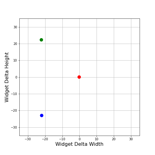
For comparison, we also plotted one of our previous samples (shown in blue) that has the same Euclidean distance from the centroid as does the green point (31.8 for both in the arbitrary units used for Delta Width and Delta Height). Can we conclude that the green point is representative of our other samples?
Clearly the answer is no, as can be seen by simply adding the other samples, shown as black points.
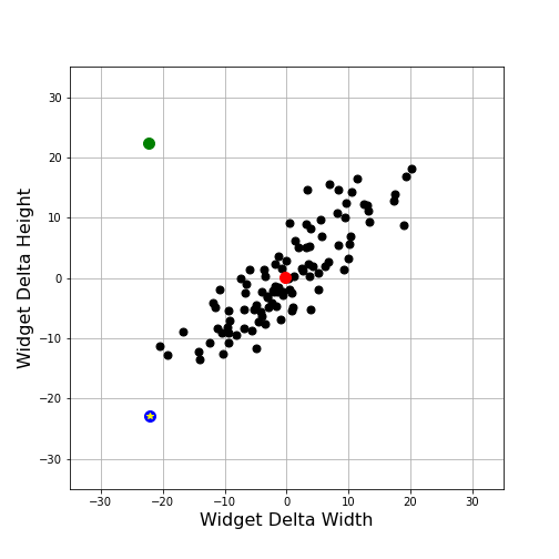
We intuitively feel that the blue point (now given an additional decoration of a yellow star) is somehow closer to cluster of black points but a computation of Z-scores doesn’t seem to help. The Z-scores for width and height for the blue point are: -2.49 and -2.82, respectively, while the corresponding values for the green point are -2.51 and 2.71.
The problem is that Delta Width and Delta Height are strongly correlated. One strategy is to follow the methods discussed in the post Multivariate Sampling and Covariance and move to a diagonalized basis. Diagonalizing the data leaves the variations expressed in an abstract space spanned by the variables X and Y, which are linear combinations of the original Delta Width and Delta Height values. The same samples plotted in these coordinates delivers the following plot.
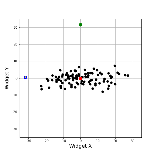
Using the X and Y coordinates as our measures, we can calculate the corresponding Z-scores for the blue point and the new green one. The X and Y Z-scores for the blue point are now: -2.74 and 0.24. These values numerically match our visual impression that the blue point, while on the outskirts of the distribution in the X-direction lies close to the centroid in the Y-direction. The corresponding X and Y Z-scores for the green point are: 0.00 and 10.16. Again, these numerical values match our visual impression that the green point is almost aligned with the centroid in the X-direction but is very far from the variation of the distribution along the Y-direction.
Before moving onto how the Mahalanobis distance handles this for us, it is worth noting that the reason the situation was so ambiguous in W-H coordinates was that when we computed the Z-scores in the W- and H- directions, we ignored the strong correlation between Delta Width and Delta Height. In doing so, we were effectively judging Z-scores in a bounding box corresponding to the maximum X- and Y-extents of the sample rather than seeing the distribution as a tightly grouped scatter about one of the bounding box’s diagonals. By going to the X-Y coordinates we were able to find the independent directions (i.e. eigendirections).
The Mahalanobis distance incorporates these notions, observations, and strategies by defining a multidimensional analog of the Z-score that is aware of the correlation between the variables. Its definition is
\[ d_M = \sqrt{ \left({\mathbf O} – {\bar {\mathbf O}} \right)^T S^{-1} \left({\mathbf O} – {\bar {\mathbf O}} \right) } \; , \]
where ${\mathbf O}$ is a column array of the values for the current point (i.e. the new, green one), ${\bar {\mathbf O}}$ is the average across the sample, and $S^{-1}$ is the inverse of the covariance matrix. Forming the radical is equivalent to calculating the square of the Z-score, which is easily seen by fact the $S^-1$ has units that are inverses of observations squared (e.g., in this case $1/length^2$). This observation also supports why the square root is needed at the end.
For the sample used in this example, the average values of W and H were: -0.172600686508044 and 0.17708029312465146. Using these gives the array
\[ {\bar {\mathbf O}} = \left[ \begin{array}{c} -0.172600686508044 \\ 0.17708029312465146 \end{array} \right] \; . \]
The covariance matrix was given by
\[ S = \left[ \begin{array}{cc} 78.29662631 & 63.08196815 \\ 63.08196815 & 67.35298221 \end{array} \right] \; . \]
The blue points observation vector is
\[ {\mathbf O}(blue) = \left[ \begin{array}{c} -22.109910673364368 \\ -22.83313653428484 \end{array} \right] \; \]
and its Mahalanobis distance from the centroid is
\[ d_M(blue) = 2.805 \; . \]
In contrast the green point as an observation vector of
\[ {\bar {\mathbf O}} = \left[ \begin{array}{c} -22.30184428079569 \\ 22.306323887412297 \end{array} \right] \; \]
giving a Mahalanobis distance from the centroid of
\[ d_M(green) = 10.142 \; . \]
Note that the magnitude of the components of blue and green observation vectors are almost identical; the critical difference being the sign on the H-component. That sign difference reflects the large deviation away from the correlation that exists in the W-H components, which shows up in the large differences in the Mahalanobis distance.
Finally, note that the Mahalanobis distance for both the blue and green point is the root-sum-square of the individual Z-scores in X-Y coordinates; this is an important point that only holds in the diagonalized coordinate system.
By exploiting the coordinate invariance of an bilinear form, the Mahalanobis distance provides the basic machinery of calculating Z-scores in the diagonalized coordinate system without the bother of actually having to carry out the diagonalization.