K-Means++ Data Clustering: Improved Seeding

This month’s column is a follow on to last month’s look at the K-means data clustering.  Again, I’ll be looking at James McCaffrey’s Test Run article K-Means++ Data Clustering, published in MSDN in August 2015.   

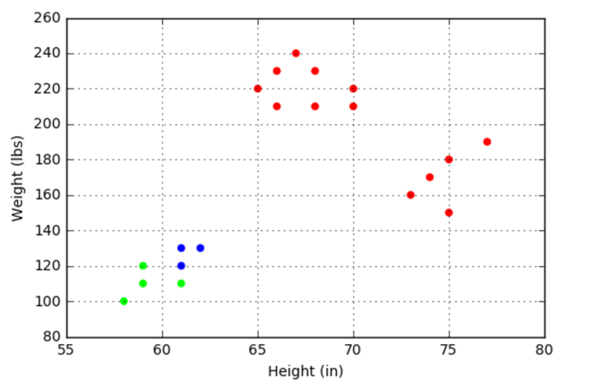
In the last post, I confined my analysis to the K-means data clustering algorithm using McCaffrey’s hand-picked data points that showed that the heights and weights of a sample of some population aggregated into 3 distinct groups of clusters.  Once the data were normalized, the human eye easily picks out these clusters but the machine, not so much.  The purpose of the K-means clustering was to provide the machine with a mechanism where it might mimic, at least in the most primitive of senses, the ability of the human eye to correlate a 2-dimensional image.

Of course, McCaffrey’s sample was designed specifically to illustrate the techniques with no gray areas that might confuse the person, let alone the computer.  Nonetheless, the algorithm failed to find the clusters completely around 20-30% of the time; an estimate of my own based on a semi-empirical method of restarting the algorithm a number of times and simply counting the number of times that the clustering gave a color-codes result that looked like the following figure (each color denoting a cluster).

The problem with the algorithm is one of seeding the process.   For each of the $k$ clusters chosen as a guess by the user, the algorithm needs to start with a guess as to where the centers of those clusters lie.  The K-means algorithm seeds the process by selecting samples from the distribution at random to give the initial guess as to the cluster centers.  If this random guess selects two nearby points as two distinct centers then a situation like the one shown above arises.

The ‘++’ in the K-means++ algorithm denotes an improvement to the seeding process to avoid this undesirable outcome.  The algorithm is called roulette wheel selection and it works as follows.

1. The first center is chosen at random
2. The distance of each remaining point, $d_{i,1}$ from this point is chosen, typically using the Euclidean norm
3. An array is formed with the cumulative sum of the $d_{i,1}$ normalized by the total $D = \sum_i d_{i,1}$ and the i^th element of the array is associated with the corresponding point
4. A random number is drawn from a uniform distribution and the first point in the array whose cumulative probability is greater than the drawn random number is chosen as the second center
5. Repeat steps 2-4 as before but using the new center rather than the old one

The roulette wheel selection implementation is not particularly hard but the are questions about performance and rather than worrying about those details, I chose to use the Kmeans roulette wheel selection implementation provided in scikit-learn since it is widely accepted and I eventually threw much larger datasets at the algorithm than the 20-element height/weight data.  Beyond the obvious import of the package (from sklearn.cluster import KMeans), the key lines for the implementation were:

kmeans_cluster = KMeans(n_clusters=<k>, n_init=<n>).fit(<data>)
point_labels = kmeans_cluster.labels_

The parameters are:

• n_clusters = <k> sets the number of clusters (aka centers or centroids) the data are believed to possess to the user-supplied value of <k>
• n_init = <n> sets the number of completely separate tries that the algorithm gets at the clustering to the user-supplied value of <n>
• <data> are the set of values in N-dimensions that are clustered

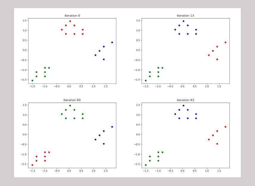
Before discussing the results, it is worth saying a few words about the n_init setting.  The default value in KMeans is 10, meaning that scikit-learn’s implementation start with fresh seeding of the clusters on 10 separate runs through the data and will keep the best one.  Since I was interested in how well the initial seeding using the Kmeans++ approach (roulette wheel selection) performed versus the traditional Kmeans approach (random selection), I set n_init = 1 for the initial testing.  Finally, I wrapped the whole process of seeding, clustering, and producing a figure into a loop with everything reset at the beginning of each pass.  In 100 trials, with n_clusters = 3, n_init = 1, and <data> being the height/weight data as before, the algorithm correctly picked out the 3 distinct clusters each time.  The randomness of the seeding was verified by the cluster color coding changing at each iteration.

While this test clearly demonstrated the improvement that the roulette wheel selection provides, it is worth noting that the seeding can’t be perfect since the algorithm can’t determine the number of clusters to begin with (the value of <k>) nor can it guarantee that the seeding process will always work (n_init = 10 as the default). 

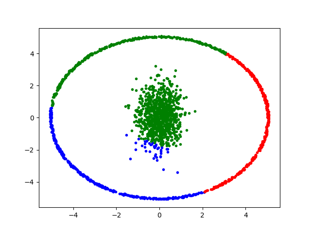
Indeed, Kmeans++ can often be fooled even when the number of the clusters is obvious and they are quite distinct from each other.  Consider the following set of points

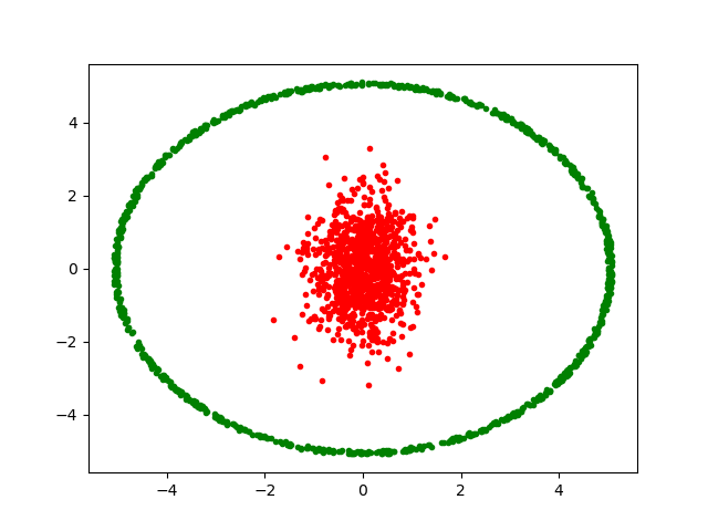
that form two distinct clusters of random realizations in two dimensions (the red from two different-sized Gaussians and the green from a tight Gaussian along the radial direction and a uniform distribution in the azimuthal direction).

Sadly, scikit-learn’s Kmeans implementation (with n_init = 10) has no apparent ability to find these clusters as seen in the following comical figures

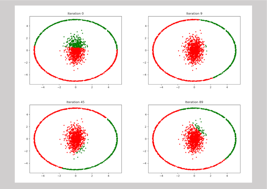
This example was derived from one of the discussion points raised in the Stack Overflow post machine learning – How to understand the drawbacks of K-means, which has lots of other examples of Kmeans coming up short.

Just for fun, I also asked Kmeans to cluster these points using n_clusters = 3 and got

which goes to show that the algorithm is really intelligent. 

To close, consider the following two points.  First, as has been pointed out by many people in many forums, no algorithm, including Kmeans++ is bulletproof.  The aphorism

best summarizes the fact that Kmeans should be only one of many tools in an ever-growing toolbox.

Second, on a humanistic vein, consider the marvelous attributes of the human being that allows a person to glance at the above figure and not only identify the number of clusters but that can also find their edges or conclude that the task is hopeless and go off for a snack.  That’s true intelligence.