
Riding a bike, catching a ball, driving a car, throwing a dart – these and countless other similar, everyday activities involve the very amazing human capacity to target. This capacity has yet to be duplicated in the machine world even in its most sophisticated applications.
To expand on this concept, take dart throwing as the prototype for analysis. In the act of hitting a bullseye, a brain, an eye, a hand, a dart, a dartboard, a throw, and a landing all come together to produce a spectacular trajectory where the missile hits exactly where the thrower intends.

How does the person learn to throw accurately? The equations governing the flight of the dart are nonlinear and subject to a variety of errors. Clearly practice and feedback from eye to brain to hand are required but how exactly does the training take hold?
While some believe that they know the answer, an honest weighing of the facts suggest that we don’t have more than an inkling into the mechanism by which intelligence and repetition interact to produce a specific skill. In Aristotelian terms, the mystery lies in how a human moves from having the potentiality to score a bullseye into being able to do it dependably.
What does seem to be clear is that this human mechanism, whatever it actually is, is quite different from any of the mathematical processes that are used in machine applications. To appreciate just how different, let’s look at one specific mathematical targeting method: differential correction.
Differential correction is the umbrella term that covers a variety of related numerical techniques, all of them based on Newton’s method. Related terms are the secant method, Newton-Raphson, the shooting method, and forward targeting. Generally speaking, these tools are used to teach a computer how to solve a set of nonlinear equations (e.g., the flight of a dart, the motion of a car, the trajectory of a rocket, etc.) that symbolically can be written as
\[ \Phi: \bar V \rightarrow \bar G \; ,\]
where $\bar V$ are the variables that we are free to manipulate and $\bar G$ are the goals we are trying to achieve. The variables are expressed in an $n$-dimensional space that, at least locally, looks like $\mathbb{R}^n$. Likewise, the goals live in an $m$-dimensional space that is also locally $\mathbb{R}^m$. The primary situation where these spaces deviate from being purely Cartesian is when some subset of the variables and/or goals are defined on a compact interval, the most typical case being when a variable is a heading angle.
These fine details and others, such as how to solve the equations when $m \neq n$, are important in practice but are not essential for this argument. The key point is that the mapping $\Phi$ only goes one way. We know how to throw the dart at the board and then see where it lands. We don’t know how to start at the desired landing point (i.e., the bullseye) and work backwards to determine how to throw. Likewise, in the mathematical setting, the equations linking the variables to the goals can’t be easily inverted.
Nonetheless, both the natural and mathematical targeting processes allow for a local inversion in the following way. Once a trial throw is made and the resulting landing point seen and understood, the initial way the dart was thrown can be modified to try to come closer. This subsequent trial informs further throws and often (although not always) the bullseye can be eventually reached.
To illustrate this in the differential correction scheme, suppose the flight of the dart depends on two variables $x$ and $y$ (the two heading angles right-to-left and up-to-down) and consider just how to solve these two equations describing where the dart lands on the board (the values of $f$ and $g$):
\[ x^2 y = f \; \]
and
\[ 2 x + \cos(y) = g \; . \]
To strike the bullseye means to solve these equations for a specified set of goals $f^*$ and $g^*$, which are the values of the desired target. There may be a clever way to solve these particular equations for $x$ and $y$ in terms of $f$ and $g$, but one can always construct so-called transcendental equations where no such analytic solution can ever be obtained (e.g. Kepler’s equation), so let’s tackle them as if no analytic form of the solution exists.
Assuming that we can find a pair of starting values $x_0$ and $y_0$ that get us close to the unknown solutions $x^*$ and $y^*$, we can ‘walk’ this first guess over to the desired initial conditions by exploiting calculus. Take the first differential of the equations
\[ 2 x y dx + x^2 dy = df \]
and
\[ 2 dx + \sin(y) dy = dg \; .\]
Next relax the idea of a differential to a finite difference – a sort of reversal of the usual limiting process by which we arrive at the calculus in the first place – and consider the differentials of the goals as the finite deviations of the target values from those achieved on the first throw: $df = f_0 – f^*$ and $dg = g_0 – g^*$. Likewise, the differential $dx = x_0 – x^*$ and $dy = y_0 – x^*$. Since we now have two linear equations in the two unknowns $x^*$ and $y^*$, we can invert to find a solution. Formally, this approach is made more obvious by combining the system into a single matrix equation
\[ \left [ \begin{array}{cc} 2 x y & x^2 \\ 2 & \sin(y) \end{array} \right] \left[ \begin{array}{c} x_0 – x^* \\ y_0 – y^* \end{array} \right] = \left[ \begin{array}{c} f_0 – f^* \\ g_0 – g^* \end{array} \right] \; .\]
The solution of this equation is then
\[ \left[ \begin{array}{c} x^* \\ y^* \end{array} \right] = \left[ \begin{array}{c} x_0 \\ y_0 \end{array} \right] – \left [ \begin{array}{cc} 2 x y & x^2 \\ 2 & \sin(y) \end{array} \right]^{-1} \left[ \begin{array}{c} f_0 – f^* \\ g_0 – g^* \end{array} \right] \; . \]
Since the original equations are non-linear, this solution is only an estimate of the actual values and, by taking these estimates as the improved guess, $x_1$ and $y_1$, an iteration scheme can be used to refine the solutions to the desired accuracy.
Everything rests on two major assumptions: 1) a sufficiently close first guess can be obtained to seed the process and 2) the equations are smooth and can be differentiated. By examining each of these assumptions, we will arrive at a keen distinction between machine and human thought.
First the idea of a first guess is so natural to us that it is often hard to even notice how crucial it is. Just how do we orient ourselves to the dartboard. The obvious answer is that we look around to find it or we ask someone else where it is. Once in sight, we then lock our attention on it and finally we throw the dart. But this description isn’t really a description at all. It lacks the depth needed to explain it to a blind person let alone explain it to the machine. In some fashion, we integrate our senses into the process in a high non-trivial way before even the first dart is thrown.
Returning to the mathematical model, consider how to find $x_0$ and $y_0$ when $f^* = 2.5$ and $g^* = 4.0$. The traditional way is to make a plot of the mapping $\Phi$, which may be considered as taking the usual Cartesian grid in $x$ and $y$ and mapping it to a set of level curves. A bit of playing with the equations leads one to the plot
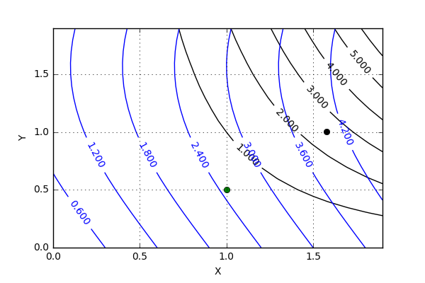
where level curves of $f$ are shown in black and those for $g$ are in blue. The trained eye can guess a starting point at or around (1.5,1.0) but, for the sake of this argument, let’s pick (1.0,0.5) (the green dot on the figure). In just a handful of iterations, the differential correction process hones in on the precise solution of (1.57829170833, 1.00361110653) (the black dot on the plot). But the mystery lies in the training of the eye and not in the calculus that follows after the first guess has been chosen. What is it about the human capacity that makes looking at the plot such an intuitive thing? Imagine trying to teach a machine to accomplish this. The machine vision algorithms needed to look at the plot and infer the first guess still don’t exist, even though the differential correction algorithm is centuries old.
Even more astonishing, once realized, is that the human experience neither deals with symbolically specified equations nor are the day-to-day physical processes for throwing darts, driving cars, or any of the myriad other things people do strictly differentiable. All of these activities are subjected to degrees of knowledge and control errors. Inexactness and noise pervade everything and yet wetware is able to adapt to extend in a way the software can’t. Somehow the human mind deals with the complexity in an emergent way that is far removed from the formal structure of calculus.
So, while it is true that the human and the machine both can target and that targeting entails trial-and-error and iteration, they do it in completely different ways. The machine process is analytic and local and limited. The human process is emergent, global, and heuristic. In addition, we can teach ourselves and others how to do it and even invent the mathematics needed to teach a pale imitation of it to computers, but we really don’t understand how.