
It is well known that developers will go to great lengths to speed up algorithms or optimize code. Performance, after all, is king. In general, accelerating throughput comes in three flavors.
The first category covers all those really sophisticated ideas that come from a clear and insightful understanding of an algorithm or a physical model.
The examples that spring to mind in the case of the algorithm are the development of the solution to the traveling salesman problem or the invention of the Fast Fourier Transform. In these cases, solutions to the problem existed but generalizing these so that they would perform well in an arbitrary setting proved to be challenging and elusive. It took decades of many dedicated people’s times to wrangle out the techniques needed to transform the elementary examples into a working technique.
A keen example of how optimization for a physical model only comes from a deep understanding of the physics is the story that Peter Lepage relayed at a seminar that I attended. The story is powerful and sticks with me to this day. At the beginning of the seminar he took moment to set aside a laptop (1990s vintage) on which he started a ‘job’. He then proceeded to talk about the evolution of Quantum Chromodynamics (QCD) in the early days after the theory had been proposed. Every few years, the team he was on would go to the NSF requesting more powerful super-computers with which to solve the QCD problem, giving in return more promises that the solution was just at hand. After 3 or 4 iterations of this loop, Lepage, said that he realized that the team had lived through something like 5 progressions of Moore’s law. The computing power had increased by a factor of roughly 32 and yet the solution remained out-of-reach. He then decided that the fault, dear Brutus, laid not in their stars but in themselves in that their algorithm was all wrong (my paraphrasing of Shakespeare not his). At this point, he interrupted the seminar and went over to the laptop. Examining it, he declared that during the time he was speaking, a small program on his machine had solved a QCD problem and had ‘discovered’ the J/Psi particle and a quark ball. He went on to explain that the performance gain he was able to create came not from better computing or large, more powerful computers, but from reworking the algorithm so that the physics (in this case renormalization) were properly considered.
In the second category, are the general optimization techniques that are taught in computer science. These involve a careful examination of how to do common things like multiplying out a polynomial, sorting a list, convolving data and so on. Counting operations and thinking about grouping and ordering are the usual ways of tackling these problems.
For example, a usual strategy to speed up polynomial evaluation is to refactor the usual way a polynomial is presented so as to minimize the number of multiplications. The fourth-order polynomial
\[ a_0 + a_1 x + a_2 x^2 + a_3 x^3 + a_4 x^4 \]
transforms into
\[ a_0 + x ( a_1 + x ( a_2 + x ( a_3 + a_4 x) ) ) \; ; \]
far less readable but far more efficient. The former case has 4 additions and 10 multiplies (assuming no calls to ‘pow’ are made). The latter case still has 4 additions but only 4 multiplies, resulting in a huge savings if the polynomial is evaluated frequently.
Another example I encountered recently centered on the binning of a large list of floating point data into a smaller array. A colleague of mine was using one of the standard scientific packages and he was amazed at the performance difference that resulted simply from changing the order of operations.
To illustrate, with a concrete case, consider the case where you have millions of floating point numbers that fall somewhere in the range between 0 and 8. In addition, you have 8 bins, labeled B0 through B7 into which to place them.
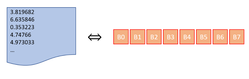 While it may seem natural, a clumsy way to place the numbers within the bins would be to pick a given bin and then traverse the list of floats finding all those that belong in that bin and then starting with the next bin and so on. This requires the traversal of the large list 8 times. A better way would be to pick a number off of the list of floats and place it into the appropriate bin, requiring only 1 movement through the list. These simple things make a huge difference but it isn’t always easy to tell how to massage a commercial piece of software into doing one versus the other.
At this point, you may be thinking that you understand the previous two categories. While you may never have the insight to contribute to the first category, you can appreciate the results. And you most likely can and will apply the techniques of the other in your day-to-day computing task. So what exactly falls into the third category?
Well, the third category comprises all of those incredible ‘tricks’ that only result from equal parts inspiration (first category), standard algorithmic understanding (second category), pride, and outright desperation.
The poster child for this category is the ‘Fast Inverse Square Root’, an algorithm that was used to perform a high-performance estimate to $1/\sqrt{x}$, since this computation is the primary one needed to normalize vectors and compute scalar products for lighting in video games.
The Wikipedia article, which gives the history, context, and analysis of the algorithm is worth reading and maybe should be mandatory for all game designers and computer scientists. I’ll not try to cover it here except to make a few observations.
First, the following figure, adapted from the Wikipedia article, shows the short set of lines needed to implement the algorithm
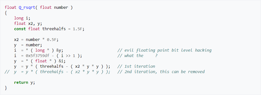
It may have been fast, but hardly maintainable. The comments (most amusing) don’t reveal much in how the algorithm works. Why, precisely, is there a cast from float to integer and what is the origin of the very specific hex value of 0x5f3759df, and to what algorithm do the lines decorated with 1st iteration and 2nd iteration refer? Apparently, the second question haunted the developer who put in the comment that I sanitized for this venue. Answers to all of these questions can be found in Wikipedia but it is worth pondering the mindset that led to the lines pictured above.
The second comment, a whimsical afterthought if you will, is the astonishing resemblance between John Carmack, credited with the fast inverse square root and Gary Cole, the actor who played Bill Lumberg in Office Space

a movie about the great lengths to which developers will go.