
Last month’s column explored the surprising complexity that results from the repeated application of the simple set of rules called the Half or Triple-Plus-One (HTPO). Despite the fact that the rules are easy to understand and apply, composing their application iteratively led to rich patterns that defy the ability of the current state of mathematical logic to fully predict or prove. So it should come as no surprise that there similar systems exhibit ‘big things in small packages’ behavior.
One class of systems where the application of simple local rules leads to complex global behavior is known as cellular automata. These systems are usually modeled as living on a grid or lattice usually with a rectangular topology, although other connection schemes exist.
The state of the system is specified by a discrete state variable living at the grid point, with the most common state being specified by the integers 0 or 1, corresponding to ‘on’ or ‘off’. The transition rules for deciding whether a grid point turns from on to off or vice versa are usually based on the local neighborhood of the grid point and are usually specified by relatively simple rules.
As in the HTPO case, the fun begins when the entire system dynamics for extended systems are taken into account. Even though a specific grid point only interacts directly with its neighbors (the precise definition of what these are differ from system to system) its future evolution is determined by its neighbor’s interactions with their neighbors and so on. In a real sense, local rules propagate out globally, and this is how the complexity results.
Perhaps the best known and popular cellular automaton system is Conway’s Game of Life. This system takes place on a rectangular grid with the state of the system specified by 0 for off (‘dead’) and 1 for on (‘alive’). Each cell has 8 neighbors, the closest cells to the north, north-east, east, south-east, south, south-west, west, and north-west. The rules for how a particular grid cell evolves in time are:
- If a cell is alive and has less than 2 neighbors, it dies from heart-crushing loneliness and a failure by society-at-large to meet its needs,
- if a cell is alive and has 2 or 3 neighbors, it flourishes due to a balanced social life where it is integrated properly into society,
- if a cell is alive and has 4 or more neighbors, it dies from overcrowding, squalor, and disease,
- and if a cell is dead but there are exactly 3 neighbors, a new baby is born to settle into the empty spot.
Of course, none of the colorful language used above is canonical. John Horton Conway picked the rules to try to balance the birth and death rates such that there would be no explosive growth and that the outcomes were not trivially predictable from the inputs. According to the Wikipedia article linked above, Conway’s work was motivated by the desire to simplify von Neumann’s invention of a computational ‘machine’ that could build copies of itself.
The introduction of the Game of Life in 1970 sparked an entire industry due to the rich, emergent patterns that result. To give a taste of the possibilities consider some simple configurations on a 6×6 grid. Perhaps the simplest, non-trivial configuration is the block, which consists of 4 cells clustered together.

Since each cell has 3 neighbors, the pattern, once established, persists into eternity and the four cells live forever together in a stable colony. Interestingly, this future-time stability does not imply past-time stability as this configuration can be reached by a variety of enormously dynamic and turbulent pasts as long as the penultimate step is a 3-cell ‘L’ configuration.
There are many stable configurations like the block. Another one that tends to appear in simulations is the beehive, which also lasts from one time to another time unless disturbed.
It is interesting to note that the addition of one extra cell anywhere where it may be counted as a neighbor to the beehive ruins the stability completely.
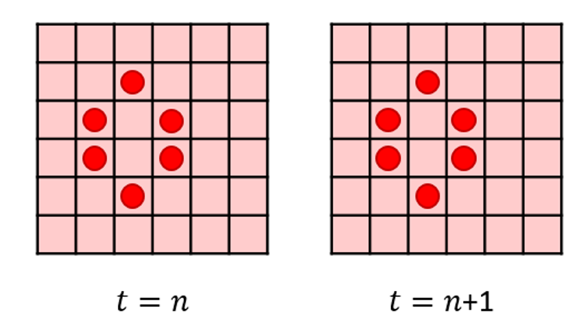
Dynamic patterns that have a stable form (really stationary) are also present, some of which are periodic and others which exhibit non-periodic, complex motions. The simplest examples of periodic behaviors are those structures that seem to spin or rotate thus seeming to retain their shape. The textbook example of this is the blinker that appears to rotate.
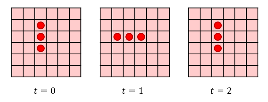
A more careful analysis shows that only the central cell persists while the exterior ones die and resurrect every second time step. The Wikipedia article shows other periodic structures, including the very beautiful pulsar, that exhibit much more complex periodicities.
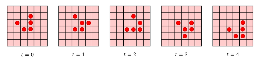
In the class of non-periodic stationary structures comes the glider, which is a 5-cell structure that sort-of shuffles its way across the board so that it walks through 4 distinct shapes such that its center moves one cell diagonally every 4 steps.
Obviously, a huge amount of complexity results from these simple rules. But the Game of Life has more structure than the emergence of a bewildering array of patterns. It turns out all logic gates needed in computing can be constructed using gliders, as seen in this video by Alex Bellos
The key structure for producing the gliders is known as Gospar’s Glider Gun, which pumps out a signal (a glider) that can be interrupted by other gliders from other guns. The fact that all possible logic gates can be constructed in the Game of Life means that it is Turing-Complete. Thus you can program any algorithm in Game of Life, including the Game of Life
Amazing what a few simple rules can do!