
Imagine that it’s Christmas Eve and, due to some poor planning on your part, you find yourself short of a few gifts – gifts for key people in your life. You reckon that you have no choice but to go out to the mall and fight all the other last minute shoppers to find those special trinkets that will bring smiles to all those faces you would rather not look at when they are frowning. You know parking will be a delicate issue with few choices available at any given time and, as you enter the lot, you happen to see a space about one foot shy of a football-field’s distance to the mall entrance. Should you take it or is there a better one closer?
If you take the space, you are in for a long walk to and fro as well as a waste of your time – and maybe, just maybe, the gifts will be gone by the time you get there. If you pass by the space you run the risk of not finding a closer space and, most likely, this space will not be there when you circle back.
In a nutshell, this type of problem is best described under the heading ‘knowing when it is time to settle’. It has broad applications in wide ranging fields; any discipline where decision making is done within the context of uncertainty mixed with a now-or-never flavor falls under this heading.
Within the computing and mathematical communities, this scenario is dubbed The Secretary Problem and has been widely studied. The article Knowing When to Stop by Theodore Hill, published by The American Scientist, presents a nice introduction and discussion of the problem within many of the real world applications. The aim of this month’s column is to look at some realizations of the problem within a computing context, and to look at some variations that lead to some interesting deviations from the common wisdom. The code and approach presented here are strongly influenced by the article The Secretary Problem by James McCaffrey in the Test Run column of MSDN Magazine. All of the code presented and all of the results were produced in a Jupyter notebook using Python 2.7 and the standard suite of numpy and matplotlib.
The basic notion of the Secretary Problem is that a company is hiring for the position of secretary and they have received a pool of applicants. Since it is expensive to interview and vet applicants and there is a lost opportunity cost for each day the position goes unfilled, the company would like to fill the position as soon as possible. On the other hand, the company doesn’t want to settle for a poor candidate if a more suitable one would be found with a bit more searching. And, overall, what expectations should the company have for the qualifications of the secretary; perhaps the market is bad all over.
Within a fairly stringent set of assumptions, there is a way to maximize the probability of selecting the best choice by using the 1/e stopping rule. To illustrate the method, imagine that 10 applicants seek the position. Divide the applicant pool up into a testing pool and a selection pool, where the size of the testing pool is determined (to within some rounding or truncation scheme) by dividing the total number of applicants by e, the base of the natural logarithms. Using truncation, the testing pool has 3 members and the selection pool has 7.

The testing pool is interviewed and the applicants assessed and scored. This sampling of the applicant pool serves to survey the entire pool. The highest score from the testing pool sets a threshold that must be met or exceeded (hopefully) by an applicant within the additional population found in the selection pool. The first applicant from the selection pool to meet or exceed the threshold is selected; this may or may not be the best overall candidate. Following this approach, and using the additional assumption that each applicant is scored uniquely, the probability is 36.8% chance of getting the best applicant (interestingly, this percentage is also 1/e).
This decision-making framework has three possible responses: it can find the best applicant, it can settle on a sub-optimal applicant, or it can fail to find any applicant that fits the bill. This later case occurs when all the best applicants are in the Testing Pool and no applicants in the Selection Pool can match or exceed the threshold.
To test the 1/e rule, I developed code in Python within the Jupyter notebook framework. The key function is the one that sets up the initial applicant pool. This function
def generate_applicants(N,flag='uniform'):
    if flag == 'integer':
        pool = []
        for i in range(0,N):
            pool.append(np.random.randint(10*N))
        return np.array(pool)
    if flag == 'normal':
        temp          = np.abs(np.random.randn(N))
        return np.floor(temp/np.max(temp)*100.0)/10.0
    if flag == 'uniform':
        return np.floor(np.random.rand(N)*100.0)/10.0
    else:
        print "Didn't understand your specification - using uniform distribution"
        return np.floor(np.random.rand(N)*100.0)/10.0
sets the scores of the applicants in one of three ways. The first method, called ‘integer’, assigns an integer to each applicant based on a uniform probability distribution. The selected range is chosen to be 10 times larger than the number of applicants, effectively guaranteeing that no two applicants have the same score. The second, called ‘normal’, assigns a score from the normal distribution. This approach also effectively guarantees that no two applicants have the same score. The occasions where both methods violate the assumption of uniqueness form a very small subset of the whole. The third method, called ‘uniform’, distributes scores uniformly but ‘quantizes’ the score to a discrete set. This last method is used to test the importance of the assumption of a unique score for each applicant.
A specific applicant pool and the application of the 1/e rule can be regarded as an individual Monte Carlo trial. Each trial is repeated a large number of times to assemble the statistics for analysis. The statistics comprise the number of times the best applicant is found, the number of times no suitable applicant is found, and the number of times a sub-optimal applicant is found and how far from the optimum said applicant is. This last statistic is called the settle value, since this is what the company has had to settle for.
The following figure shows the percentage of times that each method finds an optimal candidate from the selection pool by using the 1/e stopping rule.

Note that for the two methods where duplication is nearly impossible (integer and normal), the percent of total success remains, to within Monte Carlo error, at the theoretically derived value of about 36.8 %. In contrast, the uniform method, which enjoys a quantized scoring system, shoots upwards to a total success rate of 100%. The reason that explains this behavior is that with a quantized scoring system there is only a discrete set of values any applicant can achieve. Once the number of applicants gets great enough, the testing pool perfectly characterizes the whole. And while the number of applicants needed to achieve this higher percentage is impractical for finding a secretary (who really wants 640 applicants interviewing for the position) the application to other problems is obvious. There is really no reason that a decision process should always hinge on the difference between two choices of less than a fraction of the overall score. This fact also explains why businesses typically ‘look’ at the market and pay careful attention to who is hiring whom.
For completeness, the following figures show the analogous behavior for the partial success percentage
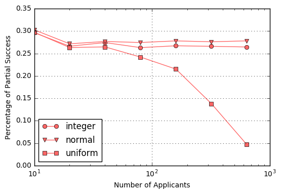
and the total failure scenarios
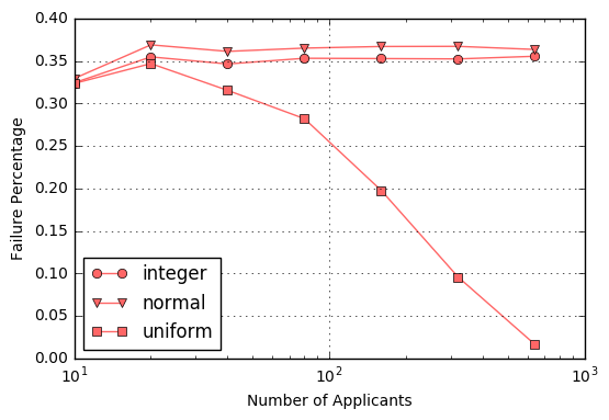
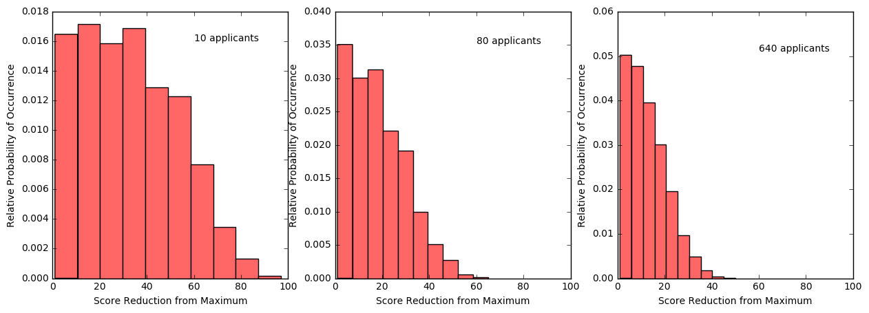
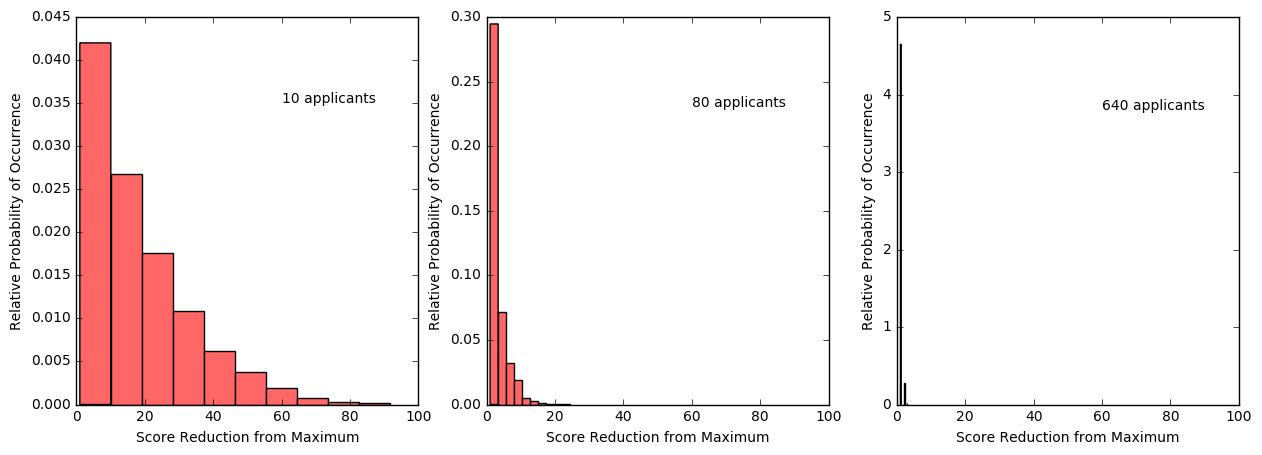
An interesting corollary is to ask, in the case of partial success, how much short of optimal did the decision process fall in the process of settling on a sub-optimal selection. The following figures shows histograms for 10, 80, and 640 applicants in the applicant pool for those cases where the decision process had to settle for a sub-optimal choice, for the normal and uniform cases, respectively. As expected, there is an improvement in how far from the maximum the decision falls as the testing pool size increases but, even with 640 applicants, the normal process has a significant probability of falling short by 20% or more.
In contrast, the distribution for the uniform scoring quickly collapses, so that the amount that the settled-upon candidate falls from the optimum is essentially within 5% even with a moderately sized applicant pool. Again, this behavior is due to the quantized scoring, which more accurately reflects real world scenarios.
At this point, there are two observations worth making in brief. First, the core assumption of the original problem, that all applicants can be assigned a unique score, is worth throwing away. Even if its adoption was crucial in deriving the 1/e stopping rule, real world applications simply do not admit a clear, unambiguous way to assign unique scores. Second, it is, perhaps, astonishing how much richness is hidden in something so mundane as hiring a qualified candidate. Of course, this is to be expected, since good help is hard to find.